ConvNet Filter Visualization
Table of Content:
Intro
Downloading the Data
First Network cats_and_dogs_small_1.h5
Data Augmentation
Second Network Using Data Augmentation: cats_and_dogs_small_2_1stlayer64.h5
Excerpt from 5.4
Own Work
Code from Chollet:
import keras
keras.__version__
'2.2.5'
5.2 - Using convnets with small datasets
This notebook contains the code sample found in Chapter 5, Section 2 of Deep Learning with Python. Note that the original text features far more content, in particular further explanations and figures: in this notebook, you will only find source code and related comments.
Training a convnet from scratch on a small dataset
Having to train an image classification model using only very little data is a common situation, which you likely encounter yourself in practice if you ever do computer vision in a professional context.
Having “few” samples can mean anywhere from a few hundreds to a few tens of thousands of images. As a practical example, we will focus on classifying images as “dogs” or “cats”, in a dataset containing 4000 pictures of cats and dogs (2000 cats, 2000 dogs). We will use 2000 pictures for training, 1000 for validation, and finally 1000 for testing.
In this section, we will review one basic strategy to tackle this problem: training a new model from scratch on what little data we have. We will start by naively training a small convnet on our 2000 training samples, without any regularization, to set a baseline for what can be achieved. This will get us to a classification accuracy of 71%. At that point, our main issue will be overfitting. Then we will introduce data augmentation, a powerful technique for mitigating overfitting in computer vision. By leveraging data augmentation, we will improve our network to reach an accuracy of 82%.
In the next section, we will review two more essential techniques for applying deep learning to small datasets: doing feature extraction with a pre-trained network (this will get us to an accuracy of 90% to 93%), and fine-tuning a pre-trained network (this will get us to our final accuracy of 95%). Together, these three strategies – training a small model from scratch, doing feature extracting using a pre-trained model, and fine-tuning a pre-trained model – will constitute your future toolbox for tackling the problem of doing computer vision with small datasets.
The relevance of deep learning for small-data problems
You will sometimes hear that deep learning only works when lots of data is available. This is in part a valid point: one fundamental characteristic of deep learning is that it is able to find interesting features in the training data on its own, without any need for manual feature engineering, and this can only be achieved when lots of training examples are available. This is especially true for problems where the input samples are very high-dimensional, like images.
However, what constitutes “lots” of samples is relative – relative to the size and depth of the network you are trying to train, for starters. It isn’t possible to train a convnet to solve a complex problem with just a few tens of samples, but a few hundreds can potentially suffice if the model is small and well-regularized and if the task is simple. Because convnets learn local, translation-invariant features, they are very data-efficient on perceptual problems. Training a convnet from scratch on a very small image dataset will still yield reasonable results despite a relative lack of data, without the need for any custom feature engineering. You will see this in action in this section.
But what’s more, deep learning models are by nature highly repurposable: you can take, say, an image classification or speech-to-text model trained on a large-scale dataset then reuse it on a significantly different problem with only minor changes. Specifically, in the case of computer vision, many pre-trained models (usually trained on the ImageNet dataset) are now publicly available for download and can be used to bootstrap powerful vision models out of very little data. That’s what we will do in the next section.
For now, let’s get started by getting our hands on the data.
Downloading the data
The cats vs. dogs dataset that we will use isn’t packaged with Keras. It was made available by Kaggle.com as part of a computer vision
competition in late 2013, back when convnets weren’t quite mainstream. You can download the original dataset at:
https://www.kaggle.com/c/dogs-vs-cats/data (you will need to create a Kaggle account if you don’t already have one – don’t worry, the
process is painless).
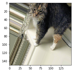
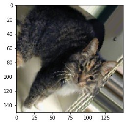
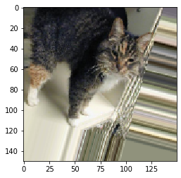
The pictures are medium-resolution color JPEGs. They look like this:
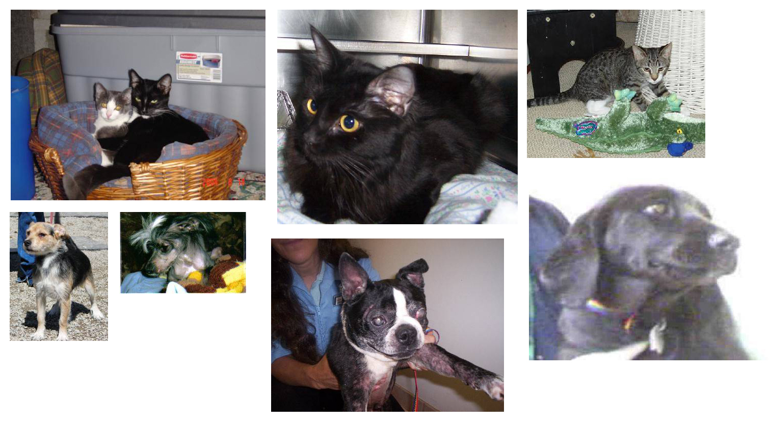
Unsurprisingly, the cats vs. dogs Kaggle competition in 2013 was won by entrants who used convnets. The best entries could achieve up to 95% accuracy. In our own example, we will get fairly close to this accuracy (in the next section), even though we will be training our models on less than 10% of the data that was available to the competitors. This original dataset contains 25,000 images of dogs and cats (12,500 from each class) and is 543MB large (compressed). After downloading and uncompressing it, we will create a new dataset containing three subsets: a training set with 1000 samples of each class, a validation set with 500 samples of each class, and finally a test set with 500 samples of each class.
Here are a few lines of code to do this:
import os, shutil
Code altered by us:
## DO NOT EXECUTE !!

# The path to the directory where the original
# dataset was uncompressed
original_dataset_dir = '/home/loecher/data/train/'

# The directory where we will
# store our smaller dataset
base_dir = '/home/loecher/data/cats_and_dogs'
os.mkdir(base_dir)

# Directories for our training,
# validation and test splits
train_dir = os.path.join(base_dir, 'train')
os.mkdir(train_dir)
validation_dir = os.path.join(base_dir, 'validation')
os.mkdir(validation_dir)
test_dir = os.path.join(base_dir, 'test')
os.mkdir(test_dir)

# Directory with our training cat pictures
train_cats_dir = os.path.join(train_dir, 'cats')
os.mkdir(train_cats_dir)

# Directory with our training dog pictures
train_dogs_dir = os.path.join(train_dir, 'dogs')
os.mkdir(train_dogs_dir)

# Directory with our validation cat pictures
validation_cats_dir = os.path.join(validation_dir, 'cats')
os.mkdir(validation_cats_dir)

# Directory with our validation dog pictures
validation_dogs_dir = os.path.join(validation_dir, 'dogs')
os.mkdir(validation_dogs_dir)

# Directory with our validation cat pictures
test_cats_dir = os.path.join(test_dir, 'cats')
os.mkdir(test_cats_dir)

# Directory with our validation dog pictures
test_dogs_dir = os.path.join(test_dir, 'dogs')
os.mkdir(test_dogs_dir)

# Copy first 1000 cat images to train_cats_dir
fnames = ['cat.{}.jpg'.format(i) for i in range(1000)]
for fname in fnames:
    src = os.path.join(original_dataset_dir, fname)
    dst = os.path.join(train_cats_dir, fname)
    shutil.copyfile(src, dst)

# Copy next 500 cat images to validation_cats_dir
fnames = ['cat.{}.jpg'.format(i) for i in range(1000, 1500)]
for fname in fnames:
    src = os.path.join(original_dataset_dir, fname)
    dst = os.path.join(validation_cats_dir, fname)
    shutil.copyfile(src, dst)

# Copy next 500 cat images to test_cats_dir
fnames = ['cat.{}.jpg'.format(i) for i in range(1500, 2000)]
for fname in fnames:
    src = os.path.join(original_dataset_dir, fname)
    dst = os.path.join(test_cats_dir, fname)
    shutil.copyfile(src, dst)

# Copy first 1000 dog images to train_dogs_dir
fnames = ['dog.{}.jpg'.format(i) for i in range(1000)]
for fname in fnames:
    src = os.path.join(original_dataset_dir, fname)
    dst = os.path.join(train_dogs_dir, fname)
    shutil.copyfile(src, dst)

# Copy next 500 dog images to validation_dogs_dir
fnames = ['dog.{}.jpg'.format(i) for i in range(1000, 1500)]
for fname in fnames:
    src = os.path.join(original_dataset_dir, fname)
    dst = os.path.join(validation_dogs_dir, fname)
    shutil.copyfile(src, dst)

# Copy next 500 dog images to test_dogs_dir
fnames = ['dog.{}.jpg'.format(i) for i in range(1500, 2000)]
for fname in fnames:
    src = os.path.join(original_dataset_dir, fname)
    dst = os.path.join(test_dogs_dir, fname)
    shutil.copyfile(src, dst)
From https://colab.research.google.com/github/google/eng-edu/blob/master/ml/pc/exercises/image_classification_part1.ipynb
#!wget --no-check-certificate \
#    https://storage.googleapis.com/mledu-datasets/cats_and_dogs_filtered.zip \
#    -O /tmp/cats_and_dogs_filtered.zip

import os
import zipfile

local_zip = 'cats_and_dogs_filtered.zip'
zip_ref = zipfile.ZipFile(local_zip, 'r')
zip_ref.extractall('/tmp')
zip_ref.close()

base_dir = '/tmp/cats_and_dogs_filtered'
train_dir = os.path.join(base_dir, 'train')
validation_dir = os.path.join(base_dir, 'validation')

# Directory with our training cat pictures
train_cats_dir = os.path.join(train_dir, 'cats')

# Directory with our training dog pictures
train_dogs_dir = os.path.join(train_dir, 'dogs')

# Directory with our validation cat pictures
validation_cats_dir = os.path.join(validation_dir, 'cats')

# Directory with our validation dog pictures
validation_dogs_dir = os.path.join(validation_dir, 'dogs')
Now, let’s see what the filenames look like in the cats and dogs train directories (file naming conventions are the same in the validation directory):
train_cat_fnames = os.listdir(train_cats_dir)
print(train_cat_fnames[:10])

train_dog_fnames = os.listdir(train_dogs_dir)
train_dog_fnames.sort()
print (train_dog_fnames[:10])
['cat.342.jpg', 'cat.491.jpg', 'cat.600.jpg', 'cat.793.jpg', 'cat.736.jpg', 'cat.77.jpg', 'cat.382.jpg', 'cat.159.jpg', 'cat.96.jpg', 'cat.826.jpg']
['dog.0.jpg', 'dog.1.jpg', 'dog.10.jpg', 'dog.100.jpg', 'dog.101.jpg', 'dog.102.jpg', 'dog.103.jpg', 'dog.104.jpg', 'dog.105.jpg', 'dog.106.jpg']
As a sanity check, let’s count how many pictures we have in each training split (train/validation/test):
print('total training cat images:', len(os.listdir(train_cats_dir)))
total training cat images: 1000
print('total training dog images:', len(os.listdir(train_dogs_dir)))
total training dog images: 1000
print('total validation cat images:', len(os.listdir(validation_cats_dir)))
total validation cat images: 500
print('total validation dog images:', len(os.listdir(validation_dogs_dir)))
total validation dog images: 500
print('total test cat images:', len(os.listdir(test_cats_dir)))
total test cat images: 500
print('total test dog images:', len(os.listdir(test_dogs_dir)))
total test dog images: 500
Code from Chollet:
So we have indeed 2000 training images, and then 1000 validation images and 1000 test images. In each split, there is the same number of samples from each class: this is a balanced binary classification problem, which means that classification accuracy will be an appropriate measure of success.
Building our network
We’ve already built a small convnet for MNIST in the previous example, so you should be familiar with them. We will reuse the same
general structure: our convnet will be a stack of alternated Conv2D (with relu activation) and MaxPooling2D layers.
However, since we are dealing with bigger images and a more complex problem, we will make our network accordingly larger: it will have one
more Conv2D + MaxPooling2D stage. This serves both to augment the capacity of the network, and to further reduce the size of the
feature maps, so that they aren’t overly large when we reach the Flatten layer. Here, since we start from inputs of size 150x150 (a
somewhat arbitrary choice), we end up with feature maps of size 7x7 right before the Flatten layer.
Note that the depth of the feature maps is progressively increasing in the network (from 32 to 128), while the size of the feature maps is decreasing (from 148x148 to 7x7). This is a pattern that you will see in almost all convnets.
Since we are attacking a binary classification problem, we are ending the network with a single unit (a Dense layer of size 1) and a
sigmoid activation. This unit will encode the probability that the network is looking at one class or the other.
from keras import layers
from keras import models

model = models.Sequential()
model.add(layers.Conv2D(32, (3, 3), activation='relu',
                        input_shape=(150, 150, 3)))
model.add(layers.MaxPooling2D((2, 2)))
model.add(layers.Conv2D(64, (3, 3), activation='relu'))
model.add(layers.MaxPooling2D((2, 2)))
model.add(layers.Conv2D(128, (3, 3), activation='relu'))
model.add(layers.MaxPooling2D((2, 2)))
model.add(layers.Conv2D(128, (3, 3), activation='relu'))
model.add(layers.MaxPooling2D((2, 2)))
model.add(layers.Flatten())
model.add(layers.Dense(512, activation='relu'))
model.add(layers.Dense(1, activation='sigmoid'))
Let’s take a look at how the dimensions of the feature maps change with every successive layer:
model.summary()
Model: "sequential_2"
_________________________________________________________________
Layer (type)                 Output Shape              Param #
=================================================================
conv2d_5 (Conv2D)            (None, 148, 148, 32)      896
_________________________________________________________________
max_pooling2d_5 (MaxPooling2 (None, 74, 74, 32)        0
_________________________________________________________________
conv2d_6 (Conv2D)            (None, 72, 72, 64)        18496
_________________________________________________________________
max_pooling2d_6 (MaxPooling2 (None, 36, 36, 64)        0
_________________________________________________________________
conv2d_7 (Conv2D)            (None, 34, 34, 128)       73856
_________________________________________________________________
max_pooling2d_7 (MaxPooling2 (None, 17, 17, 128)       0
_________________________________________________________________
conv2d_8 (Conv2D)            (None, 15, 15, 128)       147584
_________________________________________________________________
max_pooling2d_8 (MaxPooling2 (None, 7, 7, 128)         0
_________________________________________________________________
flatten_2 (Flatten)          (None, 6272)              0
_________________________________________________________________
dense_3 (Dense)              (None, 512)               3211776
_________________________________________________________________
dense_4 (Dense)              (None, 1)                 513
=================================================================
Total params: 3,453,121
Trainable params: 3,453,121
Non-trainable params: 0
_________________________________________________________________
For our compilation step, we’ll go with the RMSprop optimizer as usual. Since we ended our network with a single sigmoid unit, we will
use binary crossentropy as our loss (as a reminder, check out the table in Chapter 4, section 5 for a cheatsheet on what loss function to
use in various situations).
from keras import optimizers

model.compile(loss='binary_crossentropy',
              optimizer=optimizers.RMSprop(lr=1e-4),
              metrics=['acc'])
Data preprocessing
As you already know by now, data should be formatted into appropriately pre-processed floating point tensors before being fed into our network. Currently, our data sits on a drive as JPEG files, so the steps for getting it into our network are roughly:
- Read the picture files.
- Decode the JPEG content to RBG grids of pixels.
- Convert these into floating point tensors.
- Rescale the pixel values (between 0 and 255) to the [0, 1] interval (as you know, neural networks prefer to deal with small input values).
It may seem a bit daunting, but thankfully Keras has utilities to take care of these steps automatically. Keras has a module with image
processing helper tools, located at keras.preprocessing.image. In particular, it contains the class ImageDataGenerator which allows to
quickly set up Python generators that can automatically turn image files on disk into batches of pre-processed tensors. This is what we
will use here.
from keras.preprocessing.image import ImageDataGenerator

# All images will be rescaled by 1./255
train_datagen = ImageDataGenerator(rescale=1./255)
test_datagen = ImageDataGenerator(rescale=1./255)

train_generator = train_datagen.flow_from_directory(
        # This is the target directory
        train_dir,
        # All images will be resized to 150x150
        target_size=(150, 150),
        batch_size=20,
        # Since we use binary_crossentropy loss, we need binary labels
        class_mode='binary')

validation_generator = test_datagen.flow_from_directory(
        validation_dir,
        target_size=(150, 150),
        batch_size=20,
        class_mode='binary')
Found 2000 images belonging to 2 classes.
Found 1000 images belonging to 2 classes.
Let’s take a look at the output of one of these generators: it yields batches of 150x150 RGB images (shape (20, 150, 150, 3)) and binary
labels (shape (20,)). 20 is the number of samples in each batch (the batch size). Note that the generator yields these batches
indefinitely: it just loops endlessly over the images present in the target folder. For this reason, we need to break the iteration loop
at some point.
for data_batch, labels_batch in train_generator:
    print('data batch shape:', data_batch.shape)
    print('labels batch shape:', labels_batch.shape)
    break
data batch shape: (20, 150, 150, 3)
labels batch shape: (20,)
Let’s fit our model to the data using the generator. We do it using the fit_generator method, the equivalent of fit for data generators
like ours. It expects as first argument a Python generator that will yield batches of inputs and targets indefinitely, like ours does.
Because the data is being generated endlessly, the generator needs to know example how many samples to draw from the generator before
declaring an epoch over. This is the role of the steps_per_epoch argument: after having drawn steps_per_epoch batches from the
generator, i.e. after having run for steps_per_epoch gradient descent steps, the fitting process will go to the next epoch. In our case,
batches are 20-sample large, so it will take 100 batches until we see our target of 2000 samples.
When using fit_generator, one may pass a validation_data argument, much like with the fit method. Importantly, this argument is
allowed to be a data generator itself, but it could be a tuple of Numpy arrays as well. If you pass a generator as validation_data, then
this generator is expected to yield batches of validation data endlessly, and thus you should also specify the validation_steps argument,
which tells the process how many batches to draw from the validation generator for evaluation.
history = model.fit_generator(
      train_generator,
      steps_per_epoch=100,
      epochs=30,
      validation_data=validation_generator,
      validation_steps=50)
Epoch 1/30
100/100 [==============================] - 14s 142ms/step - loss: 0.6912 - acc: 0.5300 - val_loss: 0.6699 - val_acc: 0.5550
Epoch 2/30
100/100 [==============================] - 13s 129ms/step - loss: 0.6646 - acc: 0.6015 - val_loss: 0.6400 - val_acc: 0.6530
Epoch 3/30
100/100 [==============================] - 13s 130ms/step - loss: 0.6187 - acc: 0.6650 - val_loss: 0.6234 - val_acc: 0.6560
Epoch 4/30
100/100 [==============================] - 13s 129ms/step - loss: 0.5775 - acc: 0.6905 - val_loss: 0.6023 - val_acc: 0.6620
Epoch 5/30
100/100 [==============================] - 13s 129ms/step - loss: 0.5430 - acc: 0.7300 - val_loss: 0.5739 - val_acc: 0.6940
Epoch 6/30
100/100 [==============================] - 13s 129ms/step - loss: 0.5109 - acc: 0.7545 - val_loss: 0.5670 - val_acc: 0.7110
Epoch 7/30
100/100 [==============================] - 13s 130ms/step - loss: 0.4901 - acc: 0.7605 - val_loss: 0.5506 - val_acc: 0.7130
Epoch 8/30
100/100 [==============================] - 13s 129ms/step - loss: 0.4580 - acc: 0.7865 - val_loss: 0.5788 - val_acc: 0.7050
Epoch 9/30
100/100 [==============================] - 13s 130ms/step - loss: 0.4372 - acc: 0.7925 - val_loss: 0.5720 - val_acc: 0.7100
Epoch 10/30
100/100 [==============================] - 13s 129ms/step - loss: 0.4026 - acc: 0.8140 - val_loss: 0.5369 - val_acc: 0.7390
Epoch 11/30
100/100 [==============================] - 13s 129ms/step - loss: 0.3747 - acc: 0.8380 - val_loss: 0.5750 - val_acc: 0.7210
Epoch 12/30
100/100 [==============================] - 13s 129ms/step - loss: 0.3631 - acc: 0.8385 - val_loss: 0.5609 - val_acc: 0.7220
Epoch 13/30
100/100 [==============================] - 13s 133ms/step - loss: 0.3323 - acc: 0.8600 - val_loss: 0.5541 - val_acc: 0.7410
Epoch 14/30
100/100 [==============================] - 13s 129ms/step - loss: 0.3055 - acc: 0.8730 - val_loss: 0.5806 - val_acc: 0.7380
Epoch 15/30
100/100 [==============================] - 13s 129ms/step - loss: 0.2784 - acc: 0.8900 - val_loss: 0.5717 - val_acc: 0.7420
Epoch 16/30
100/100 [==============================] - 13s 129ms/step - loss: 0.2559 - acc: 0.8990 - val_loss: 0.6133 - val_acc: 0.7190
Epoch 17/30
100/100 [==============================] - 13s 127ms/step - loss: 0.2286 - acc: 0.9140 - val_loss: 0.6063 - val_acc: 0.7400
Epoch 18/30
100/100 [==============================] - 13s 128ms/step - loss: 0.2013 - acc: 0.9250 - val_loss: 0.6103 - val_acc: 0.7490
Epoch 19/30
100/100 [==============================] - 13s 128ms/step - loss: 0.1799 - acc: 0.9340 - val_loss: 0.6704 - val_acc: 0.7370
Epoch 20/30
100/100 [==============================] - 13s 131ms/step - loss: 0.1615 - acc: 0.9455 - val_loss: 0.6941 - val_acc: 0.7270
Epoch 21/30
100/100 [==============================] - 13s 130ms/step - loss: 0.1362 - acc: 0.9485 - val_loss: 0.6813 - val_acc: 0.7390
Epoch 22/30
100/100 [==============================] - 13s 129ms/step - loss: 0.1198 - acc: 0.9615 - val_loss: 0.7462 - val_acc: 0.7360
Epoch 23/30
100/100 [==============================] - 13s 131ms/step - loss: 0.1076 - acc: 0.9615 - val_loss: 0.7300 - val_acc: 0.7470
Epoch 24/30
100/100 [==============================] - 13s 129ms/step - loss: 0.0926 - acc: 0.9735 - val_loss: 0.8897 - val_acc: 0.7240
Epoch 25/30
100/100 [==============================] - 13s 129ms/step - loss: 0.0876 - acc: 0.9725 - val_loss: 0.7537 - val_acc: 0.7460
Epoch 26/30
100/100 [==============================] - 13s 129ms/step - loss: 0.0651 - acc: 0.9815 - val_loss: 0.7918 - val_acc: 0.7330
Epoch 27/30
100/100 [==============================] - 13s 134ms/step - loss: 0.0563 - acc: 0.9860 - val_loss: 0.9026 - val_acc: 0.7370
Epoch 28/30
100/100 [==============================] - 13s 130ms/step - loss: 0.0470 - acc: 0.9860 - val_loss: 0.9057 - val_acc: 0.7410
Epoch 29/30
100/100 [==============================] - 13s 130ms/step - loss: 0.0371 - acc: 0.9900 - val_loss: 1.5699 - val_acc: 0.6740
Epoch 30/30
100/100 [==============================] - 13s 129ms/step - loss: 0.0287 - acc: 0.9945 - val_loss: 1.0836 - val_acc: 0.7310
It is good practice to always save your models after training:
model.save('cats_and_dogs_small_1.h5')
Let’s plot the loss and accuracy of the model over the training and validation data during training:
import matplotlib.pyplot as plt

acc = history.history['acc']
val_acc = history.history['val_acc']
loss = history.history['loss']
val_loss = history.history['val_loss']

epochs = range(len(acc))

plt.plot(epochs, acc, 'bo', label='Training acc')
plt.plot(epochs, val_acc, 'b', label='Validation acc')
plt.title('Training and validation accuracy')
plt.legend()

plt.figure()

plt.plot(epochs, loss, 'bo', label='Training loss')
plt.plot(epochs, val_loss, 'b', label='Validation loss')
plt.title('Training and validation loss')
plt.legend()

plt.show()
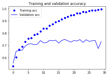
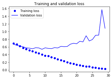
These plots are characteristic of overfitting. Our training accuracy increases linearly over time, until it reaches nearly 100%, while our validation accuracy stalls at 70-72%. Our validation loss reaches its minimum after only five epochs then stalls, while the training loss keeps decreasing linearly until it reaches nearly 0.
Because we only have relatively few training samples (2000), overfitting is going to be our number one concern. You already know about a number of techniques that can help mitigate overfitting, such as dropout and weight decay (L2 regularization). We are now going to introduce a new one, specific to computer vision, and used almost universally when processing images with deep learning models: data augmentation.
Using data augmentation
Overfitting is caused by having too few samples to learn from, rendering us unable to train a model able to generalize to new data. Given infinite data, our model would be exposed to every possible aspect of the data distribution at hand: we would never overfit. Data augmentation takes the approach of generating more training data from existing training samples, by “augmenting” the samples via a number of random transformations that yield believable-looking images. The goal is that at training time, our model would never see the exact same picture twice. This helps the model get exposed to more aspects of the data and generalize better.
In Keras, this can be done by configuring a number of random transformations to be performed on the images read by our ImageDataGenerator
instance. Let’s get started with an example:
datagen = ImageDataGenerator(
      rotation_range=40,
      width_shift_range=0.2,
      height_shift_range=0.2,
      shear_range=0.2,
      zoom_range=0.2,
      horizontal_flip=True,
      fill_mode='nearest')
These are just a few of the options available (for more, see the Keras documentation). Let’s quickly go over what we just wrote:
rotation_rangeis a value in degrees (0-180), a range within which to randomly rotate pictures.width_shiftandheight_shiftare ranges (as a fraction of total width or height) within which to randomly translate pictures vertically or horizontally.shear_rangeis for randomly applying shearing transformations.zoom_rangeis for randomly zooming inside pictures.horizontal_flipis for randomly flipping half of the images horizontally – relevant when there are no assumptions of horizontal asymmetry (e.g. real-world pictures).fill_modeis the strategy used for filling in newly created pixels, which can appear after a rotation or a width/height shift.
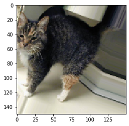
Let’s take a look at our augmented images:
Code from us:
train_cats_dir = '/home/loecher/data/cats_and_dogs/train/cats'
Code from Chollet:
import matplotlib.pyplot as plt

# This is module with image preprocessing utilities
from keras.preprocessing import image

fnames = [os.path.join(train_cats_dir, fname) for fname in os.listdir(train_cats_dir)]

# We pick one image to "augment"
img_path = fnames[3]

# Read the image and resize it
img = image.load_img(img_path, target_size=(150, 150))

# Convert it to a Numpy array with shape (150, 150, 3)
x = image.img_to_array(img)

# Reshape it to (1, 150, 150, 3)
x = x.reshape((1,) + x.shape)

# The .flow() command below generates batches of randomly transformed images.
# It will loop indefinitely, so we need to `break` the loop at some point!
i = 0
for batch in datagen.flow(x, batch_size=1):
    plt.figure(i)
    imgplot = plt.imshow(image.array_to_img(batch[0]))
    #some_batches.append(batch[0])
    i += 1
    if i % 4 == 0: # Number of pictures printed
        break

plt.show()
If we train a new network using this data augmentation configuration, our network will never see twice the same input. However, the inputs that it sees are still heavily intercorrelated, since they come from a small number of original images – we cannot produce new information, we can only remix existing information. As such, this might not be quite enough to completely get rid of overfitting. To further fight overfitting, we will also add a Dropout layer to our model, right before the densely-connected classifier:
Code altered by us:
model = models.Sequential()
model.add(layers.Conv2D(64, (3, 3), activation='relu',
                        input_shape=(150, 150, 3))) # NOTE: 32 was changed to 64 to run the 5.4.2 code (due to 8x8)
model.add(layers.MaxPooling2D((2, 2)))
model.add(layers.Conv2D(64, (3, 3), activation='relu'))
model.add(layers.MaxPooling2D((2, 2)))
model.add(layers.Conv2D(128, (3, 3), activation='relu'))
model.add(layers.MaxPooling2D((2, 2)))
model.add(layers.Conv2D(128, (3, 3), activation='relu'))
model.add(layers.MaxPooling2D((2, 2)))
model.add(layers.Flatten())
model.add(layers.Dropout(0.5))
model.add(layers.Dense(512, activation='relu'))
model.add(layers.Dense(1, activation='sigmoid'))

model.compile(loss='binary_crossentropy',
              optimizer=optimizers.RMSprop(lr=1e-4),
              metrics=['acc'])
WARNING:tensorflow:From /home/jupyter-loecher/.local/lib/python3.6/site-packages/keras/backend/tensorflow_backend.py:3733: calling dropout (from tensorflow.python.ops.nn_ops) with keep_prob is deprecated and will be removed in a future version.
Instructions for updating:
Please use `rate` instead of `keep_prob`. Rate should be set to `rate = 1 - keep_prob`.
model.summary()
Let’s train our network using data augmentation and dropout:
import time
start_time = time.time()

train_datagen = ImageDataGenerator(
    rescale=1./255,
    rotation_range=40,
    width_shift_range=0.2,
    height_shift_range=0.2,
    shear_range=0.2,
    zoom_range=0.2,
    horizontal_flip=True,)

# Note that the validation data should not be augmented!
test_datagen = ImageDataGenerator(rescale=1./255)

train_generator = train_datagen.flow_from_directory(
        # This is the target directory
        train_dir,
        # All images will be resized to 150x150
        target_size=(150, 150),
        batch_size=32,
        # Since we use binary_crossentropy loss, we need binary labels
        class_mode='binary')

validation_generator = test_datagen.flow_from_directory(
        validation_dir,
        target_size=(150, 150),
        batch_size=32,
        class_mode='binary')

history1 = model.fit_generator(
      train_generator,
      steps_per_epoch=100,
      epochs=100,
      validation_data=validation_generator,
      validation_steps=50)

print("--- %s seconds ---" % (time.time() - start_time))
Found 2000 images belonging to 2 classes.
Found 1000 images belonging to 2 classes.
Epoch 1/100
100/100 [==============================] - 33s 332ms/step - loss: 0.6929 - acc: 0.5069 - val_loss: 0.6797 - val_acc: 0.6225
Epoch 2/100
100/100 [==============================] - 32s 323ms/step - loss: 0.6836 - acc: 0.5528 - val_loss: 0.6695 - val_acc: 0.5445
Epoch 3/100
100/100 [==============================] - 32s 320ms/step - loss: 0.6605 - acc: 0.5900 - val_loss: 0.6880 - val_acc: 0.5508
Epoch 4/100
100/100 [==============================] - 33s 333ms/step - loss: 0.6472 - acc: 0.6162 - val_loss: 0.6043 - val_acc: 0.6611
Epoch 5/100
100/100 [==============================] - 33s 326ms/step - loss: 0.6335 - acc: 0.6381 - val_loss: 0.5840 - val_acc: 0.6999
Epoch 6/100
100/100 [==============================] - 33s 333ms/step - loss: 0.6081 - acc: 0.6684 - val_loss: 0.5662 - val_acc: 0.6965
Epoch 7/100
100/100 [==============================] - 32s 322ms/step - loss: 0.6076 - acc: 0.6634 - val_loss: 0.6079 - val_acc: 0.6669
Epoch 8/100
100/100 [==============================] - 33s 327ms/step - loss: 0.5951 - acc: 0.6772 - val_loss: 0.5732 - val_acc: 0.6920
Epoch 9/100
100/100 [==============================] - 33s 325ms/step - loss: 0.5885 - acc: 0.6787 - val_loss: 0.5581 - val_acc: 0.7049
Epoch 10/100
100/100 [==============================] - 32s 324ms/step - loss: 0.5830 - acc: 0.6956 - val_loss: 0.5384 - val_acc: 0.7297
Epoch 11/100
100/100 [==============================] - 33s 331ms/step - loss: 0.5717 - acc: 0.7041 - val_loss: 0.5280 - val_acc: 0.7339
Epoch 12/100
100/100 [==============================] - 32s 323ms/step - loss: 0.5709 - acc: 0.7003 - val_loss: 0.5590 - val_acc: 0.7189
Epoch 13/100
100/100 [==============================] - 33s 329ms/step - loss: 0.5503 - acc: 0.7178 - val_loss: 0.5429 - val_acc: 0.7081
Epoch 14/100
100/100 [==============================] - 32s 323ms/step - loss: 0.5535 - acc: 0.7144 - val_loss: 0.5094 - val_acc: 0.7398
Epoch 15/100
100/100 [==============================] - 33s 326ms/step - loss: 0.5485 - acc: 0.7147 - val_loss: 0.5164 - val_acc: 0.7384
Epoch 16/100
100/100 [==============================] - 33s 325ms/step - loss: 0.5545 - acc: 0.7247 - val_loss: 0.5038 - val_acc: 0.7416
Epoch 17/100
100/100 [==============================] - 32s 321ms/step - loss: 0.5358 - acc: 0.7356 - val_loss: 0.5695 - val_acc: 0.7005
Epoch 18/100
100/100 [==============================] - 33s 332ms/step - loss: 0.5333 - acc: 0.7303 - val_loss: 0.5289 - val_acc: 0.7146
Epoch 19/100
100/100 [==============================] - 32s 322ms/step - loss: 0.5302 - acc: 0.7341 - val_loss: 0.5381 - val_acc: 0.7278
Epoch 20/100
100/100 [==============================] - 33s 329ms/step - loss: 0.5270 - acc: 0.7347 - val_loss: 0.5041 - val_acc: 0.7487
Epoch 21/100
100/100 [==============================] - 33s 326ms/step - loss: 0.5155 - acc: 0.7419 - val_loss: 0.5013 - val_acc: 0.7360
Epoch 22/100
100/100 [==============================] - 33s 330ms/step - loss: 0.5147 - acc: 0.7487 - val_loss: 0.4922 - val_acc: 0.7481
Epoch 23/100
100/100 [==============================] - 33s 327ms/step - loss: 0.5207 - acc: 0.7403 - val_loss: 0.4722 - val_acc: 0.7773
Epoch 24/100
100/100 [==============================] - 33s 335ms/step - loss: 0.5121 - acc: 0.7494 - val_loss: 0.5078 - val_acc: 0.7242
Epoch 25/100
100/100 [==============================] - 33s 326ms/step - loss: 0.4991 - acc: 0.7556 - val_loss: 0.4839 - val_acc: 0.7564
Epoch 26/100
100/100 [==============================] - 32s 323ms/step - loss: 0.5049 - acc: 0.7497 - val_loss: 0.4686 - val_acc: 0.7697
Epoch 27/100
100/100 [==============================] - 33s 326ms/step - loss: 0.4985 - acc: 0.7519 - val_loss: 0.4874 - val_acc: 0.7526
Epoch 28/100
100/100 [==============================] - 32s 324ms/step - loss: 0.4917 - acc: 0.7638 - val_loss: 0.4585 - val_acc: 0.7849
Epoch 29/100
100/100 [==============================] - 33s 330ms/step - loss: 0.4992 - acc: 0.7550 - val_loss: 0.4599 - val_acc: 0.7706
Epoch 30/100
100/100 [==============================] - 32s 323ms/step - loss: 0.4930 - acc: 0.7669 - val_loss: 0.4794 - val_acc: 0.7589
Epoch 31/100
100/100 [==============================] - 33s 332ms/step - loss: 0.4862 - acc: 0.7628 - val_loss: 0.4952 - val_acc: 0.7590
Epoch 32/100
100/100 [==============================] - 33s 327ms/step - loss: 0.4813 - acc: 0.7731 - val_loss: 0.4881 - val_acc: 0.7674
Epoch 33/100
100/100 [==============================] - 32s 322ms/step - loss: 0.4781 - acc: 0.7678 - val_loss: 0.4455 - val_acc: 0.7811
Epoch 34/100
100/100 [==============================] - 33s 327ms/step - loss: 0.4874 - acc: 0.7647 - val_loss: 0.4454 - val_acc: 0.7777
Epoch 35/100
100/100 [==============================] - 32s 325ms/step - loss: 0.4614 - acc: 0.7844 - val_loss: 0.4549 - val_acc: 0.7709
Epoch 36/100
100/100 [==============================] - 33s 327ms/step - loss: 0.4806 - acc: 0.7678 - val_loss: 0.4447 - val_acc: 0.7848
Epoch 37/100
100/100 [==============================] - 33s 326ms/step - loss: 0.4578 - acc: 0.7866 - val_loss: 0.4859 - val_acc: 0.7633
Epoch 38/100
100/100 [==============================] - 33s 325ms/step - loss: 0.4620 - acc: 0.7834 - val_loss: 0.4957 - val_acc: 0.7506
Epoch 39/100
100/100 [==============================] - 32s 316ms/step - loss: 0.4671 - acc: 0.7750 - val_loss: 0.4496 - val_acc: 0.7709
Epoch 40/100
100/100 [==============================] - 32s 319ms/step - loss: 0.4585 - acc: 0.7819 - val_loss: 0.4252 - val_acc: 0.8048
Epoch 41/100
100/100 [==============================] - 31s 315ms/step - loss: 0.4513 - acc: 0.7850 - val_loss: 0.4123 - val_acc: 0.8112
Epoch 42/100
100/100 [==============================] - 31s 314ms/step - loss: 0.4493 - acc: 0.7853 - val_loss: 0.4439 - val_acc: 0.7900
Epoch 43/100
100/100 [==============================] - 32s 317ms/step - loss: 0.4519 - acc: 0.7881 - val_loss: 0.4723 - val_acc: 0.7764
Epoch 44/100
100/100 [==============================] - 31s 315ms/step - loss: 0.4528 - acc: 0.7984 - val_loss: 0.4604 - val_acc: 0.7944
Epoch 45/100
100/100 [==============================] - 32s 321ms/step - loss: 0.4408 - acc: 0.7922 - val_loss: 0.4939 - val_acc: 0.7655
Epoch 46/100
100/100 [==============================] - 32s 315ms/step - loss: 0.4314 - acc: 0.7941 - val_loss: 0.4741 - val_acc: 0.7824
Epoch 47/100
100/100 [==============================] - 32s 320ms/step - loss: 0.4569 - acc: 0.7850 - val_loss: 0.4532 - val_acc: 0.8003
Epoch 48/100
100/100 [==============================] - 33s 327ms/step - loss: 0.4452 - acc: 0.7928 - val_loss: 0.4462 - val_acc: 0.7938
Epoch 49/100
100/100 [==============================] - 32s 322ms/step - loss: 0.4371 - acc: 0.7941 - val_loss: 0.4722 - val_acc: 0.7709
Epoch 50/100
100/100 [==============================] - 33s 328ms/step - loss: 0.4392 - acc: 0.7972 - val_loss: 0.4109 - val_acc: 0.8170
Epoch 51/100
100/100 [==============================] - 32s 323ms/step - loss: 0.4325 - acc: 0.7953 - val_loss: 0.4556 - val_acc: 0.7773
Epoch 52/100
100/100 [==============================] - 33s 333ms/step - loss: 0.4304 - acc: 0.8072 - val_loss: 0.4085 - val_acc: 0.8054
Epoch 53/100
100/100 [==============================] - 32s 323ms/step - loss: 0.4323 - acc: 0.7978 - val_loss: 0.4501 - val_acc: 0.7963
Epoch 54/100
100/100 [==============================] - 33s 329ms/step - loss: 0.4230 - acc: 0.8044 - val_loss: 0.4171 - val_acc: 0.8067
Epoch 55/100
100/100 [==============================] - 33s 327ms/step - loss: 0.4337 - acc: 0.7969 - val_loss: 0.4104 - val_acc: 0.8077
Epoch 56/100
100/100 [==============================] - 33s 331ms/step - loss: 0.4178 - acc: 0.7991 - val_loss: 0.4154 - val_acc: 0.7970
Epoch 57/100
100/100 [==============================] - 33s 331ms/step - loss: 0.4217 - acc: 0.8078 - val_loss: 0.4754 - val_acc: 0.7629
Epoch 58/100
100/100 [==============================] - 32s 324ms/step - loss: 0.4026 - acc: 0.8175 - val_loss: 0.4186 - val_acc: 0.7963
Epoch 59/100
100/100 [==============================] - 33s 328ms/step - loss: 0.4203 - acc: 0.8028 - val_loss: 0.4006 - val_acc: 0.8170
Epoch 60/100
100/100 [==============================] - 33s 327ms/step - loss: 0.4315 - acc: 0.8019 - val_loss: 0.4089 - val_acc: 0.7938
Epoch 61/100
100/100 [==============================] - 33s 327ms/step - loss: 0.4166 - acc: 0.8034 - val_loss: 0.4611 - val_acc: 0.7841
Epoch 62/100
100/100 [==============================] - 33s 326ms/step - loss: 0.4199 - acc: 0.8041 - val_loss: 0.4204 - val_acc: 0.8090
Epoch 63/100
100/100 [==============================] - 33s 328ms/step - loss: 0.3987 - acc: 0.8197 - val_loss: 0.3999 - val_acc: 0.8196
Epoch 64/100
100/100 [==============================] - 32s 324ms/step - loss: 0.4065 - acc: 0.8194 - val_loss: 0.4110 - val_acc: 0.8189
Epoch 65/100
100/100 [==============================] - 32s 323ms/step - loss: 0.3994 - acc: 0.8222 - val_loss: 0.4073 - val_acc: 0.8185
Epoch 66/100
100/100 [==============================] - 33s 328ms/step - loss: 0.3938 - acc: 0.8269 - val_loss: 0.4619 - val_acc: 0.7912
Epoch 67/100
 84/100 [========================>.....] - ETA: 4s - loss: 0.4150 - acc: 0.8073


---------------------------------------------------------------------------

KeyboardInterrupt                         Traceback (most recent call last)

<ipython-input-50-c8e1df54bd6d> in <module>
     33       epochs=100,
     34       validation_data=validation_generator,
---> 35       validation_steps=50)
     36
     37 print("--- %s seconds ---" % (time.time() - start_time))


~/.local/lib/python3.6/site-packages/keras/legacy/interfaces.py in wrapper(*args, **kwargs)
     89                 warnings.warn('Update your `' + object_name + '` call to the ' +
     90                               'Keras 2 API: ' + signature, stacklevel=2)
---> 91             return func(*args, **kwargs)
     92         wrapper._original_function = func
     93         return wrapper


~/.local/lib/python3.6/site-packages/keras/engine/training.py in fit_generator(self, generator, steps_per_epoch, epochs, verbose, callbacks, validation_data, validation_steps, validation_freq, class_weight, max_queue_size, workers, use_multiprocessing, shuffle, initial_epoch)
   1656             use_multiprocessing=use_multiprocessing,
   1657             shuffle=shuffle,
-> 1658             initial_epoch=initial_epoch)
   1659
   1660     @interfaces.legacy_generator_methods_support


~/.local/lib/python3.6/site-packages/keras/engine/training_generator.py in fit_generator(model, generator, steps_per_epoch, epochs, verbose, callbacks, validation_data, validation_steps, validation_freq, class_weight, max_queue_size, workers, use_multiprocessing, shuffle, initial_epoch)
    213                 outs = model.train_on_batch(x, y,
    214                                             sample_weight=sample_weight,
--> 215                                             class_weight=class_weight)
    216
    217                 outs = to_list(outs)


~/.local/lib/python3.6/site-packages/keras/engine/training.py in train_on_batch(self, x, y, sample_weight, class_weight)
   1447             ins = x + y + sample_weights
   1448         self._make_train_function()
-> 1449         outputs = self.train_function(ins)
   1450         return unpack_singleton(outputs)
   1451


~/.local/lib/python3.6/site-packages/keras/backend/tensorflow_backend.py in __call__(self, inputs)
   2977                     return self._legacy_call(inputs)
   2978
-> 2979             return self._call(inputs)
   2980         else:
   2981             if py_any(is_tensor(x) for x in inputs):


~/.local/lib/python3.6/site-packages/keras/backend/tensorflow_backend.py in _call(self, inputs)
   2935             fetched = self._callable_fn(*array_vals, run_metadata=self.run_metadata)
   2936         else:
-> 2937             fetched = self._callable_fn(*array_vals)
   2938         return fetched[:len(self.outputs)]
   2939


~/.local/lib/python3.6/site-packages/tensorflow/python/client/session.py in __call__(self, *args, **kwargs)
   1456         ret = tf_session.TF_SessionRunCallable(self._session._session,
   1457                                                self._handle, args,
-> 1458                                                run_metadata_ptr)
   1459         if run_metadata:
   1460           proto_data = tf_session.TF_GetBuffer(run_metadata_ptr)


KeyboardInterrupt:
print("Run time:", round(3165.070887565613/60, 2), "minutes.")
Let’s save our model – we will be using it in the section on convnet visualization.
model.save('cats_and_dogs_small_2_1stlayer64.h5')
import matplotlib.pyplot as plt

acc = history1.history['acc']
val_acc = history1.history['val_acc']
loss = history1.history['loss']
val_loss = history1.history['val_loss']

epochs = range(len(acc))

plt.plot(epochs, acc, 'bo', label='Training acc')
plt.plot(epochs, val_acc, 'b', label='Validation acc')
plt.title('Training and validation accuracy')
plt.legend()

plt.figure()

plt.plot(epochs, loss, 'bo', label='Training loss')
plt.plot(epochs, val_loss, 'b', label='Validation loss')
plt.title('Training and validation loss')
plt.legend()

plt.show()
#!cp cats_and_dogs_small_2.h5 cats_and_dogs_small_2_1stlayer64.h5
Code from us:
Small and Large Neural Networks:
We have two Neural Networks, one small and one large.
Overview (Go To):
Libraries
Functions
Small Neural Network
Large Neural Network
import functools
from operator import mul

from keras.preprocessing import image
from keras.preprocessing.image import ImageDataGenerator
from keras import backend as K
from keras import models
from keras.applications import VGG16

import tensorflow as tf

import pandas as pd
import numpy as np
import matplotlib.pyplot as plt

import time

import lightgbm as lgb

from sklearn.metrics import accuracy_score
from sklearn.metrics import confusion_matrix
Functions: Small and Large Neural Networks
#1: This function (written by Chollet) deprocesses the image.
def deprocess_image(x):
    # normalize tensor: center on 0., ensure std is 0.1
    x -= x.mean()
    x /= (x.std() + 1e-5)
    x *= 0.1

    # clip to [0, 1]
    x += 0.5
    x = np.clip(x, 0, 1)

    # convert to RGB array
    x *= 255
    x = np.clip(x, 0, 255).astype('uint8')
    return x
#2: This function (written by Chollet) creates an image tensor representing the pattern that maximizes the activation the specified filter.
def generate_pattern(model, layer_name, filter_index, size=150):
    # Build a loss function that maximizes the activation
    # of the nth filter of the layer considered.
    layer_output = model.get_layer(layer_name).output
    loss = K.mean(layer_output[:, :, :, filter_index])

    # Compute the gradient of the input picture wrt this loss
    grads = K.gradients(loss, model.input)[0]

    # Normalization trick: we normalize the gradient
    grads /= (K.sqrt(K.mean(K.square(grads))) + 1e-5)

    # This function returns the loss and grads given the input picture
    iterate = K.function([model.input], [loss, grads])

    # We start from a gray image with some noise
    input_img_data = np.random.random((1, size, size, 3)) * 20 + 128.

    # Run gradient ascent for 40 steps
    step = 1.
    for i in range(40):
        loss_value, grads_value = iterate([input_img_data])
        input_img_data += grads_value * step

    img = input_img_data[0]
    return deprocess_image(img)
#3 This function (partly taken from Chollet) generates training and validation data.
def gen_train_valid_data():
    from keras.preprocessing import image

    # Training part

    datagen = ImageDataGenerator(
      rotation_range=40,
      width_shift_range=0.2,
      height_shift_range=0.2,
      shear_range=0.2,
      zoom_range=0.2,
      horizontal_flip=True,
      fill_mode='nearest')

    all_augmented_pictures = []
    for animal in ['cat', 'dog']:
        for i in range(1000): # number of cats pictures in the following folder
            # For Local Server:
            #img_path = '/Users/Nik/Documents/CodeAndStats/deep-learning-with-python-notebooks-master-2/train/' + animal +'s/' + animal + '.' + str(i) + '.jpg'
            # For Plato Server:
            img_path = '/home/loecher/data/cats_and_dogs/train/' + animal +'s/' + animal + '.' + str(i) + '.jpg'

            # Read the image and resize it
            img = image.load_img(img_path, target_size=(150, 150))

            # Convert it to a Numpy array with shape (150, 150, 3)
            x = image.img_to_array(img)

            # Reshape it to (1, 150, 150, 3)
            x = x.reshape((1,) + x.shape)

            # The .flow() command below generates batches of randomly transformed images.
            # It will loop indefinitely, so we need to `break` the loop at some point!
            i = 0
            for batch in datagen.flow(x, batch_size=1):
                #plt.figure(i)
                #imgplot = plt.imshow(image.array_to_img(batch[0]))
                #all_augmented_pictures.append(batch[0]/255.) # NOTE: probably has to be resized
                all_augmented_pictures.append(np.expand_dims(image.array_to_img(batch[0]), axis = 0)/255.)
                i += 1
                if i % 4 == 0: # Number of pictures printed
                    break

    # Validation part
    validation_pictures = []

    for animal in ['cat', 'dog']:
        for i in range(1000,1500): # number of cats pictures in the following folder
            # For Local Server:
            #img_path = '/Users/Nik/Documents/CodeAndStats/deep-learning-with-python-notebooks-master-2/validation/' + animal +'s/' + animal + '.' + str(i) + '.jpg'
            # For Plato Server:
            img_path = '/home/loecher/data/cats_and_dogs/validation/' + animal +'s/' + animal + '.' + str(i) + '.jpg'
            # This is module with image preprocessing utilities
            from keras.preprocessing import image

            # Read the image and resize it
            img = image.load_img(img_path, target_size=(150, 150))

            # Convert it to a Numpy array with shape (150, 150, 3)
            x = image.img_to_array(img)

            # Reshape it to (1, 150, 150, 3)
            x = x.reshape((1,) + x.shape)

            x /= 255.

            validation_pictures.append(x)

    return(all_augmented_pictures, validation_pictures)
#4 This function (not taken from Chollet) generates the predictions, put in a flattened matrix using Keras. See here for details.
def flat_matrices(model, index, train_img, validation_img):

    # Training
    flattened_matrix = []
    for i in range(len(train_img)):
        predicts_train = model.predict(train_img[i])[index]
        predicts_train_shape = functools.reduce(mul, predicts_train.shape)
        flattened_matrix.append(np.reshape(predicts_train, predicts_train_shape))
    flattened_matrix_np = np.vstack(flattened_matrix)

    # Validation
    flattened_matrix_valid = []
    for i in range(len(validation_img)):
        predicts_valid = model.predict(validation_img[i])[index]
        predicts_valid_shape = functools.reduce(mul, predicts_valid.shape)
        flattened_matrix_valid.append(np.reshape(predicts_valid, predicts_valid_shape))
    flattened_matrix_valid_np = np.vstack(flattened_matrix_valid)

    # Cats are 0
    # Dogs are 1
    train_labels = [0] * 4000 + [1] * 4000

    # Cats are 0
    # Dogs are 1
    validation_labels = [0] * 500 + [1] * 500

    layer_shape_output = model.layers[index].output_shape

    print("Layer name:", model.layers[index].name)
    print("Output shape:", model.layers[index].output_shape)
    return(flattened_matrix_np, flattened_matrix_valid_np, train_labels, validation_labels, layer_shape_output)
#5 This function (not taken from Chollet) uses LightGBM to generate the Feature Importances. It returns the top n features (top_n_features) and the dimension (top_n_dimensions) they are in.
def acc_and_features(iterations, train, validation, validations_labels, train_label, layer_shapes, l_rate = 0.05, depth = 4, n_features = 100):

    d_train = lgb.Dataset(train, label = train_label)

    # parameter
    params = {}
    params['learning_rate'] = l_rate
    params['boosting_type'] = 'gbdt'
    params['objective'] = 'binary'
    params['metric'] = 'binary_logloss'
    params['sub_feature'] = 1 # keep at 1 for Boosting only
    params['num_leaves'] = 10
    params['min_data'] = 50
    params['max_depth'] = depth
    #params['max_bin'] = 10
    params['bagging_fraction'] = 0.25

    clf = lgb.train(params, d_train, iterations) # trains

    y_pred = clf.predict(validation) # predicts

    top_n_features = clf.feature_importance("gain").argsort()[-n_features:][::-1] # returns top n features positions
    top_n_dimensions = top_n_features % layer_shapes[-1]
    unique, counts = np.unique(top_n_dimensions, return_counts=True)
    top_n_dimensions_df = pd.DataFrame({'label': unique, 'Counts': counts}).sort_values("Counts", ascending=False)

    print("Training shape:", train.shape)
    print("The accuracy is:", accuracy_score(np.round(y_pred), validations_labels))
    return(top_n_features, top_n_dimensions, top_n_dimensions_df)
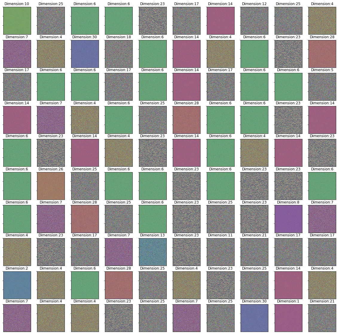
#6 This function (not taken from Chollet) plots the top n dimensions (top_dimensions).
def plot_dimensions(model, top_dimensions, index = 8):
    w = 5
    h = 5
    fig = plt.figure(figsize=(20, 20))
    columns = 5
    rows = 5

    # ax enables access to manipulate each of subplots
    ax = []
    cols = int(len(top_dimensions)/10)
    # for i in range(columns*rows):
    for i in range(len(top_dimensions)):
        # create subplot and append to ax
        #ax.append(fig.add_subplot(rows, columns, i+1))
        ax.append(fig.add_subplot(10, cols, i+1))
        ax[-1].set_title("Dimension:" + str(top_dimensions[i]))  # set title
        ax[-1].set_yticklabels([])
        ax[-1].set_xticklabels([])
        ax[-1].set_xticks([])
        ax[-1].set_xticks([])
        plt.imshow(generate_pattern(model, model.layers[index].name, top_dimensions[i]))

    #ax[2].plot(xs, 3*ys)
    #ax[19].plot(ys**2, xs)

    plt.show()  # finally, render the plot
#7 This function (not taken from Chollet) combines the previous functions. It may be used, but it is slow.
def run_all(model, index = 8, iteration = 1000, features = 100):
    all_augmented_pictures, validation_pictures = gen_train_valid_data()
    train_matrices, validation_matrices, train_labels, valid_labels, layer_shape = flat_matrices(model, index, all_augmented_pictures, validation_pictures)
    top_features, top_dimensions, top_dim_counts = acc_and_features(iterations = iteration,
                                                            train = train_matrices,
                                                            validation = validation_matrices,
                                                            validations_labels = valid_labels,
                                                            train_label = train_labels,
                                                            layer_shapes = layer_shape,
                                                            depth = 4,
                                                            n_features = features)
    plot_dimensions(model, top_dimensions = top_dimensions, index = index)
#7.1 Alternatively the functions can be called independently.
all_augmented_pictures, validation_pictures = gen_train_valid_data()
train_matrices, validation_matrices, train_labels, valid_labels, layer_shape = flat_matrices(model, index, all_augmented_pictures, validation_pictures)
top_features, top_dimensions, top_dim_counts = acc_and_features(iterations = iteration,
                                                            train = train_matrices,
                                                            validation = validation_matrices,
                                                            validations_labels = valid_labels,
                                                            train_label = train_labels,
                                                            layer_shapes = layer_shape,
                                                            depth = 4,
                                                            n_features = features)
plot_dimensions(model, top_dimensions = top_dimensions, index = index)
Small Neural Network:
Go To: Overview
Go To: Large Neural Network
from keras.models import load_model
model_small = load_model('cats_and_dogs_small_2_1stlayer32.h5')
“In order to extract the feature maps we want to look at, we will create a Keras model that takes batches of images as input, and outputs the activations of all convolution and pooling layers. To do this, we will use the Keras class Model. A Model is instantiated using two arguments: an input tensor (or list of input tensors), and an output tensor (or list of output tensors). The resulting class is a Keras model, just like the Sequential models that you are familiar with, mapping the specified inputs to the specified outputs. What sets the Model class apart is that it allows for models with multiple outputs, unlike Sequential. For more information about the Model class, see Chapter 7, Section 1.” (Chollet, Notebook 5.4)
# Extracts the outputs of the top 8 layers:
layer_outputs = [layer.output for layer in model_small.layers[:8]]
# Creates a model that will return these outputs, given the model input:
activation_model_small = models.Model(inputs=model_small.input, outputs=layer_outputs)
model_small.summary()
Model: "sequential_6"
_________________________________________________________________
Layer (type)                 Output Shape              Param #
=================================================================
conv2d_21 (Conv2D)           (None, 148, 148, 32)      896
_________________________________________________________________
max_pooling2d_21 (MaxPooling (None, 74, 74, 32)        0
_________________________________________________________________
conv2d_22 (Conv2D)           (None, 72, 72, 64)        18496
_________________________________________________________________
max_pooling2d_22 (MaxPooling (None, 36, 36, 64)        0
_________________________________________________________________
conv2d_23 (Conv2D)           (None, 34, 34, 128)       73856
_________________________________________________________________
max_pooling2d_23 (MaxPooling (None, 17, 17, 128)       0
_________________________________________________________________
conv2d_24 (Conv2D)           (None, 15, 15, 128)       147584
_________________________________________________________________
max_pooling2d_24 (MaxPooling (None, 7, 7, 128)         0
_________________________________________________________________
flatten_6 (Flatten)          (None, 6272)              0
_________________________________________________________________
dropout_5 (Dropout)          (None, 6272)              0
_________________________________________________________________
dense_11 (Dense)             (None, 512)               3211776
_________________________________________________________________
dense_12 (Dense)             (None, 1)                 513
=================================================================
Total params: 3,453,121
Trainable params: 3,453,121
Non-trainable params: 0
_________________________________________________________________
activation_model_small.summary()
Model: "model_1"
_________________________________________________________________
Layer (type)                 Output Shape              Param #
=================================================================
conv2d_21_input (InputLayer) (None, 150, 150, 3)       0
_________________________________________________________________
conv2d_21 (Conv2D)           (None, 148, 148, 32)      896
_________________________________________________________________
max_pooling2d_21 (MaxPooling (None, 74, 74, 32)        0
_________________________________________________________________
conv2d_22 (Conv2D)           (None, 72, 72, 64)        18496
_________________________________________________________________
max_pooling2d_22 (MaxPooling (None, 36, 36, 64)        0
_________________________________________________________________
conv2d_23 (Conv2D)           (None, 34, 34, 128)       73856
_________________________________________________________________
max_pooling2d_23 (MaxPooling (None, 17, 17, 128)       0
_________________________________________________________________
conv2d_24 (Conv2D)           (None, 15, 15, 128)       147584
_________________________________________________________________
max_pooling2d_24 (MaxPooling (None, 7, 7, 128)         0
=================================================================
Total params: 240,832
Trainable params: 240,832
Non-trainable params: 0
_________________________________________________________________
# This is the output shape of the activation_model_small
activation_model_small.output_shape
[(None, 148, 148, 32),
 (None, 74, 74, 32),
 (None, 72, 72, 64),
 (None, 36, 36, 64),
 (None, 34, 34, 128),
 (None, 17, 17, 128),
 (None, 15, 15, 128),
 (None, 7, 7, 128)]
Small Neural Network: Images
Images: First Layer
all_augmented_pictures, validation_pictures = gen_train_valid_data()
train_matrices, validation_matrices, train_labels, valid_labels, layer_shape = flat_matrices(activation_model_small, 1,
                                                                                             all_augmented_pictures,
                                                                                             validation_pictures)
Layer name: conv2d_21
Output shape: (None, 148, 148, 32)
top_features, top_dimensions, top_dim_counts = acc_and_features(iterations = 1000,
                                                            train = train_matrices,
                                                            validation = validation_matrices,
                                                            validations_labels = valid_labels,
                                                            train_label = train_labels,
                                                            layer_shapes = layer_shape,
                                                            depth = 4,
                                                            n_features = 100)
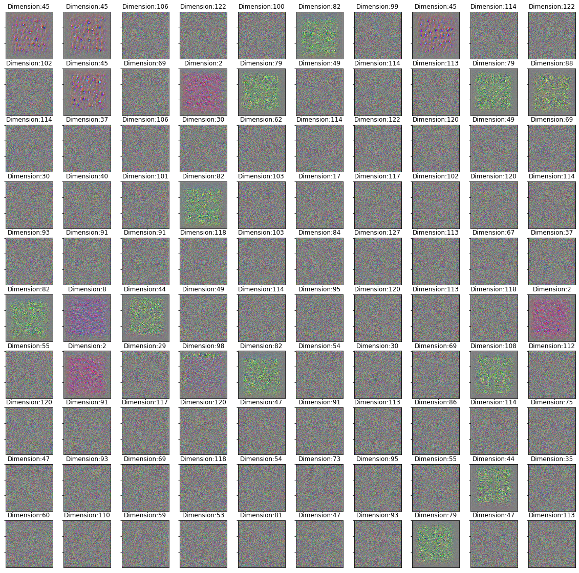
Training shape: (8000, 175232)
The accuracy is: 0.687
plot_dimensions(activation_model_small, top_dimensions = top_dimensions, index = 1)
Images: Eigth Layer
train_matrices, validation_matrices, train_labels, valid_labels, layer_shape = flat_matrices(activation_model_small, 7,
                                                                                             all_augmented_pictures,
                                                                                             validation_pictures)
Layer name: conv2d_24
Output shape: (None, 15, 15, 128)
top_features, top_dimensions, top_dim_counts = acc_and_features(iterations = 1000,
                                                            train = train_matrices,
                                                            validation = validation_matrices,
                                                            validations_labels = valid_labels,
                                                            train_label = train_labels,
                                                            layer_shapes = layer_shape,
                                                            depth = 4,
                                                            n_features = 100)
Training shape: (8000, 6272)
The accuracy is: 0.809
plot_dimensions(activation_model_small, top_dimensions = top_dimensions, index = 7)
Images: First Layer run_all
start_time = time.time()
run_all(activation_model_small, 1, 100, 10)
print("--- %s seconds ---" % (time.time() - start_time))
Layer name: conv2d_21
Output shape: (None, 148, 148, 32)
Large Neural Network:
Go To: Overview
Go To: Small Neural Network
from keras.applications import VGG16
model_large = VGG16(weights='imagenet',
              include_top=False,
             input_shape=(150, 150, 3))
“In order to extract the feature maps we want to look at, we will create a Keras model that takes batches of images as input, and outputs the activations of all convolution and pooling layers. To do this, we will use the Keras class Model. A Model is instantiated using two arguments: an input tensor (or list of input tensors), and an output tensor (or list of output tensors). The resulting class is a Keras model, just like the Sequential models that you are familiar with, mapping the specified inputs to the specified outputs. What sets the Model class apart is that it allows for models with multiple outputs, unlike Sequential. For more information about the Model class, see Chapter 7, Section 1.” (Chollet, Notebook 5.4)
# Extracts the outputs of the top n layers:
layer_outputs_large = [layer.output for layer in model_large.layers[:16]]
# Creates a model that will return these outputs, given the model input:
activation_model_large = models.Model(inputs = model_large.input, outputs = layer_outputs_large[1:]) # skip input layer
model_large.summary()
Model: "vgg16"
_________________________________________________________________
Layer (type)                 Output Shape              Param #
=================================================================
input_2 (InputLayer)         (None, 150, 150, 3)       0
_________________________________________________________________
block1_conv1 (Conv2D)        (None, 150, 150, 64)      1792
_________________________________________________________________
block1_conv2 (Conv2D)        (None, 150, 150, 64)      36928
_________________________________________________________________
block1_pool (MaxPooling2D)   (None, 75, 75, 64)        0
_________________________________________________________________
block2_conv1 (Conv2D)        (None, 75, 75, 128)       73856
_________________________________________________________________
block2_conv2 (Conv2D)        (None, 75, 75, 128)       147584
_________________________________________________________________
block2_pool (MaxPooling2D)   (None, 37, 37, 128)       0
_________________________________________________________________
block3_conv1 (Conv2D)        (None, 37, 37, 256)       295168
_________________________________________________________________
block3_conv2 (Conv2D)        (None, 37, 37, 256)       590080
_________________________________________________________________
block3_conv3 (Conv2D)        (None, 37, 37, 256)       590080
_________________________________________________________________
block3_pool (MaxPooling2D)   (None, 18, 18, 256)       0
_________________________________________________________________
block4_conv1 (Conv2D)        (None, 18, 18, 512)       1180160
_________________________________________________________________
block4_conv2 (Conv2D)        (None, 18, 18, 512)       2359808
_________________________________________________________________
block4_conv3 (Conv2D)        (None, 18, 18, 512)       2359808
_________________________________________________________________
block4_pool (MaxPooling2D)   (None, 9, 9, 512)         0
_________________________________________________________________
block5_conv1 (Conv2D)        (None, 9, 9, 512)         2359808
_________________________________________________________________
block5_conv2 (Conv2D)        (None, 9, 9, 512)         2359808
_________________________________________________________________
block5_conv3 (Conv2D)        (None, 9, 9, 512)         2359808
_________________________________________________________________
block5_pool (MaxPooling2D)   (None, 4, 4, 512)         0
=================================================================
Total params: 14,714,688
Trainable params: 14,714,688
Non-trainable params: 0
_________________________________________________________________
activation_model_large.summary()
Model: "model_1"
_________________________________________________________________
Layer (type)                 Output Shape              Param #
=================================================================
input_2 (InputLayer)         (None, 150, 150, 3)       0
_________________________________________________________________
block1_conv1 (Conv2D)        (None, 150, 150, 64)      1792
_________________________________________________________________
block1_conv2 (Conv2D)        (None, 150, 150, 64)      36928
_________________________________________________________________
block1_pool (MaxPooling2D)   (None, 75, 75, 64)        0
_________________________________________________________________
block2_conv1 (Conv2D)        (None, 75, 75, 128)       73856
_________________________________________________________________
block2_conv2 (Conv2D)        (None, 75, 75, 128)       147584
_________________________________________________________________
block2_pool (MaxPooling2D)   (None, 37, 37, 128)       0
_________________________________________________________________
block3_conv1 (Conv2D)        (None, 37, 37, 256)       295168
_________________________________________________________________
block3_conv2 (Conv2D)        (None, 37, 37, 256)       590080
_________________________________________________________________
block3_conv3 (Conv2D)        (None, 37, 37, 256)       590080
_________________________________________________________________
block3_pool (MaxPooling2D)   (None, 18, 18, 256)       0
_________________________________________________________________
block4_conv1 (Conv2D)        (None, 18, 18, 512)       1180160
_________________________________________________________________
block4_conv2 (Conv2D)        (None, 18, 18, 512)       2359808
_________________________________________________________________
block4_conv3 (Conv2D)        (None, 18, 18, 512)       2359808
_________________________________________________________________
block4_pool (MaxPooling2D)   (None, 9, 9, 512)         0
_________________________________________________________________
block5_conv1 (Conv2D)        (None, 9, 9, 512)         2359808
=================================================================
Total params: 9,995,072
Trainable params: 9,995,072
Non-trainable params: 0
_________________________________________________________________
# This is the output shape of the activation_model_small
activation_model_large.output_shape
[(None, 150, 150, 64),
 (None, 150, 150, 64),
 (None, 75, 75, 64),
 (None, 75, 75, 128),
 (None, 75, 75, 128),
 (None, 37, 37, 128),
 (None, 37, 37, 256),
 (None, 37, 37, 256),
 (None, 37, 37, 256),
 (None, 18, 18, 256),
 (None, 18, 18, 512),
 (None, 18, 18, 512),
 (None, 18, 18, 512),
 (None, 9, 9, 512),
 (None, 9, 9, 512)]
Large Neural Network: Images
Images: 14th Layer
start_time = time.time()
all_augmented_pictures, validation_pictures = gen_train_valid_data()
print("--- %s seconds ---" % (time.time() - start_time))
--- 41.29212760925293 seconds ---
start_time = time.time()
train_matrices, validation_matrices, train_labels, valid_labels, layer_shape = flat_matrices(activation_model_large,
                                                                                             14,
                                                                                             all_augmented_pictures,
                                                                                             validation_pictures)
print("--- %s seconds ---" % (time.time() - start_time))
Layer name: block4_pool
Output shape: (None, 9, 9, 512)
--- 295.3232398033142 seconds ---
start_time = time.time()
top_features, top_dimensions, top_dim_counts = acc_and_features(iterations = 1000,
                                                            train = train_matrices,
                                                            validation = validation_matrices,
                                                            validations_labels = valid_labels,
                                                            train_label = train_labels,
                                                            layer_shapes = layer_shape,
                                                            depth = 4,
                                                            n_features = 50)
print("--- %s seconds ---" % (time.time() - start_time))
Training shape: (8000, 41472)
The accuracy is: 0.896
--- 237.72960710525513 seconds ---
start_time = time.time()
import matplotlib.pyplot as plt
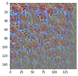
plt.imshow(generate_pattern(activation_model_large, activation_model_large.layers[14].name, 14))
print("The max. Dimension for this Layer is:", layer_shape[-1])
print("The name of the Layer is:", activation_model_large.layers[1].name)
plt.show()
print("--- %s seconds ---" % (time.time() - start_time))
The max. Dimension for this Layer is: 512
The name of the Layer is: block1_conv1
--- 3.4397711753845215 seconds ---
hundred_dims = np.arange(0,60)
start_time = time.time()
plot_dimensions(activation_model_large, hundred_dims, index = 14)
print("--- %s seconds ---" % (time.time() - start_time))
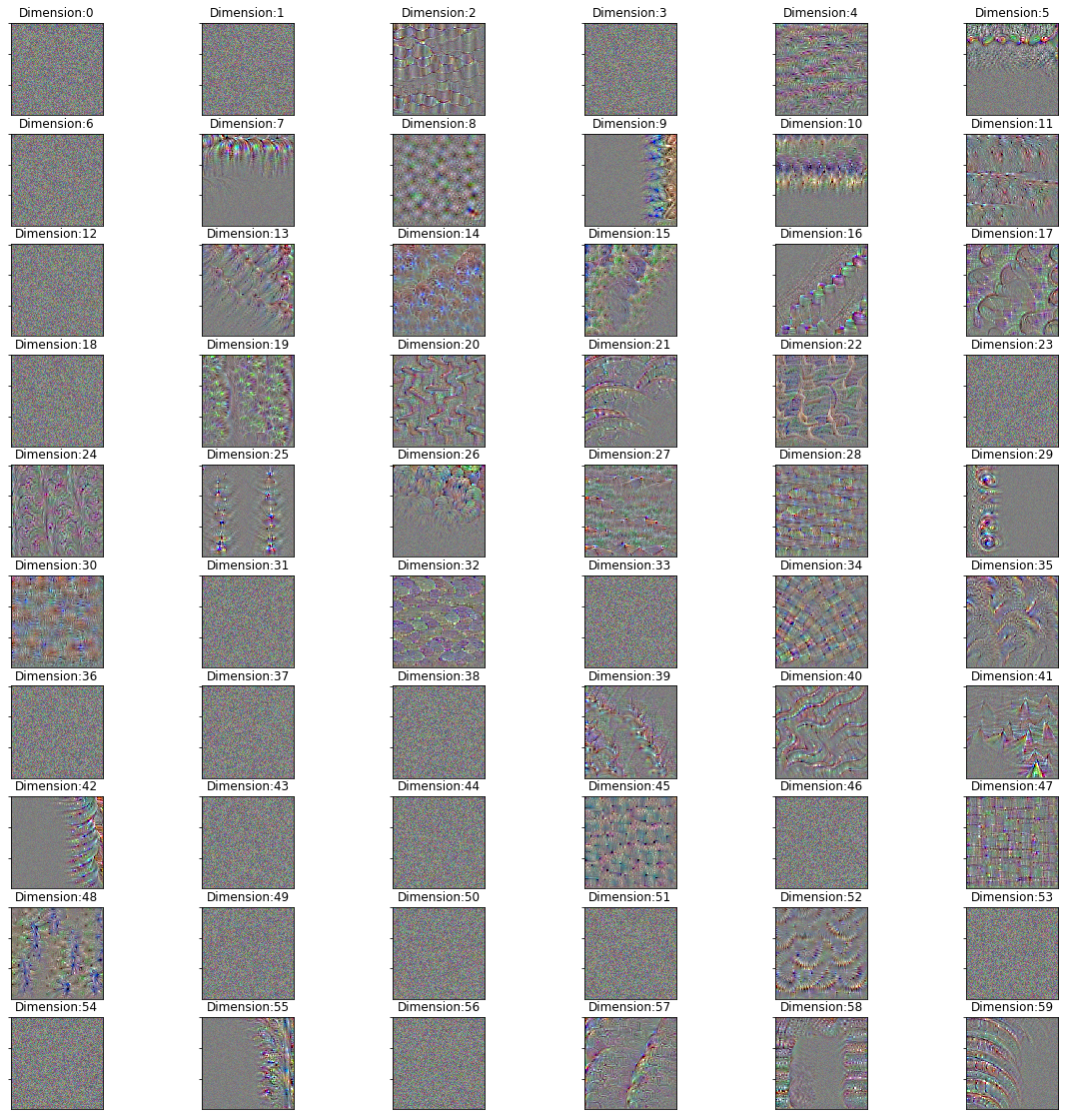
--- 210.06499481201172 seconds ---
Images: Eleventh Layer
start_time = time.time()
all_augmented_pictures, validation_pictures = gen_train_valid_data()
print("--- %s seconds ---" % (time.time() - start_time))
--- 43.48359417915344 seconds ---
start_time = time.time()
train_matrices, validation_matrices, train_labels, valid_labels, layer_shape = flat_matrices(activation_model_large,
                                                                                             11,
                                                                                             all_augmented_pictures,
                                                                                             validation_pictures)
print("--- %s seconds ---" % (time.time() - start_time))
Layer name: block4_conv1
Output shape: (None, 18, 18, 512)
--- 297.40040254592896 seconds ---
start_time = time.time()
top_features, top_dimensions, top_dim_counts = acc_and_features(iterations = 100,
                                                            train = train_matrices,
                                                            validation = validation_matrices,
                                                            validations_labels = valid_labels,
                                                            train_label = train_labels,
                                                            layer_shapes = layer_shape,
                                                            depth = 4,
                                                            n_features = 10)
print("--- %s seconds ---" % (time.time() - start_time))
Training shape: (8000, 165888)
The accuracy is: 0.802
--- 274.7301445007324 seconds ---
def acc_and_features(iterations, train, validation, validations_labels, train_label, layer_shapes, l_rate = 0.05, depth = 4, n_features = 100):

    d_train = lgb.Dataset(train, label = train_label)

    # parameter
    params = {}
    params['learning_rate'] = l_rate
    params['boosting_type'] = 'gbdt'
    params['objective'] = 'binary'
    params['metric'] = 'binary_logloss'
    params['sub_feature'] = 1 # keep at 1 for Boosting only
    params['num_leaves'] = 10
    params['min_data'] = 50
    params['max_depth'] = depth
    #params['max_bin'] = 10
    params['bagging_fraction'] = 0.25

    clf = lgb.train(params, d_train, iterations) # trains

    y_pred = clf.predict(validation) # predicts

    top_n_features = clf.feature_importance("gain").argsort()[-n_features:][::-1] # returns top n features positions
    top_n_dimensions = top_n_features % layer_shapes[-1]
    unique, counts = np.unique(top_n_dimensions, return_counts=True)
    top_n_dimensions_df = pd.DataFrame({'label': unique, 'Counts': counts}).sort_values("Counts", ascending=False)

    print("Training shape:", train.shape)
    print("The accuracy is:", accuracy_score(np.round(y_pred), validations_labels))
    return(top_n_features, top_n_dimensions, top_n_dimensions_df)
Features & Dimensions:
Features: top_features are the top n features.
top_features
array([11541, 20565, 34461,   458, 16376, 12149, 20974, 25121, 21496,
       26094,  7778, 15911, 16820, 11301, 39069,  3384, 25592, 25738,
        5944, 26199,  1848, 20022,  7029, 30365, 12212, 10277, 15909,
       25173, 21891, 11303,  4554, 20814, 28829,  7534, 25080, 20472,
        6751, 34746, 26104,  9178, 37270,  3896, 29731, 25987, 39581,
       12158, 12280,  6471, 21558, 17714])
print(activation_model_large.output_shape[11])
print(18*18*512)
(None, 18, 18, 512)
165888
Dimensions: top_dimensions are the respective dimensions to the features. For example, if there are 512 dimensions in one layer, every 512th feature is in the same dimension.
top_dimensions
array([277,  85, 157, 458, 504, 373, 494,  33, 504, 494,  98,  39, 436,
        37, 157, 312, 504, 138, 312,  87, 312,  54, 373, 157, 436,  37,
        37,  85, 387,  39, 458, 334, 157, 366, 504, 504,  95, 442, 504,
       474, 406, 312,  35, 387, 157, 382, 504, 327,  54, 306])
activation_model_large.output_shape[11]
(None, 18, 18, 512)
Plot:
start_time = time.time()
plot_dimensions(activation_model_large, top_dimensions, index = 11)
print("--- %s seconds ---" % (time.time() - start_time))
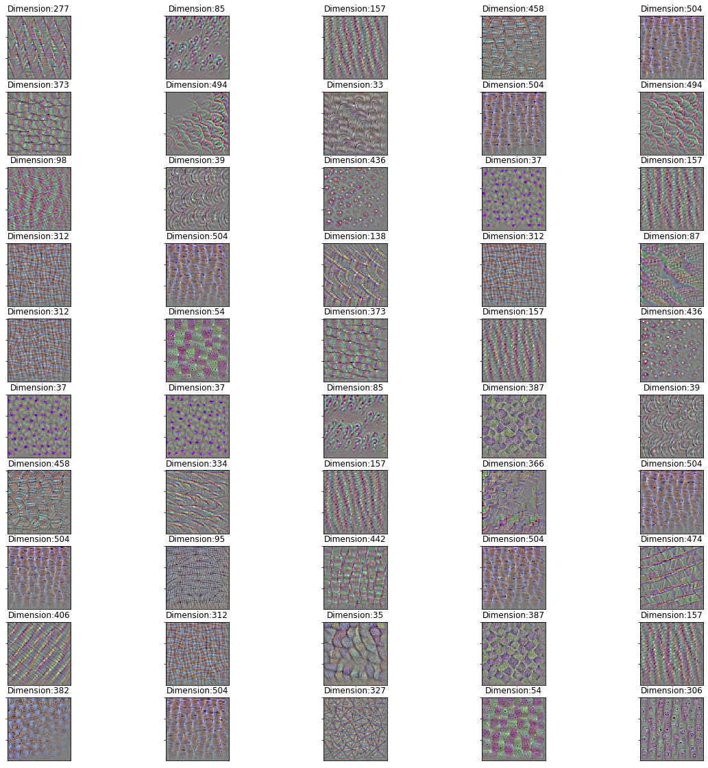
--- 203.75928449630737 seconds ---
Images: Only one Dimension
start_time = time.time()

import matplotlib.pyplot as plt
plt.imshow(generate_pattern(activation_model_large, activation_model_large.layers[11].name, top_dimensions[2]))
print("The max. Dimension for this Layer is:", layer_shape[-1])
print("The name of the Layer is:", activation_model_large.layers[11].name)
plt.show()

print("--- %s seconds ---" % (time.time() - start_time))
Images: Eleventh Layer run_all
start_time = time.time()
run_all(activation_model_large, 11, 1000, 100)
print("--- %s seconds ---" % (time.time() - start_time))
Layer name: block4_conv1
Output shape: (None, 18, 18, 512)
Training shape: (8000, 165888)
The accuracy is: 0.847
Call Python Function
%run CNN-plot.py
%load CNN-plot.py
Code from Chollet:
Let’s plot our results again:
acc = history.history['acc']
val_acc = history.history['val_acc']
loss = history.history['loss']
val_loss = history.history['val_loss']

epochs = range(len(acc))

plt.plot(epochs, acc, 'bo', label='Training acc')
plt.plot(epochs, val_acc, 'b', label='Validation acc')
plt.title('Training and validation accuracy')
plt.legend()

plt.figure()

plt.plot(epochs, loss, 'bo', label='Training loss')
plt.plot(epochs, val_loss, 'b', label='Validation loss')
plt.title('Training and validation loss')
plt.legend()

plt.show()
Thanks to data augmentation and dropout, we are no longer overfitting: the training curves are rather closely tracking the validation curves. We are now able to reach an accuracy of 82%, a 15% relative improvement over the non-regularized model.
By leveraging regularization techniques even further and by tuning the network’s parameters (such as the number of filters per convolution layer, or the number of layers in the network), we may be able to get an even better accuracy, likely up to 86-87%. However, it would prove very difficult to go any higher just by training our own convnet from scratch, simply because we have so little data to work with. As a next step to improve our accuracy on this problem, we will have to leverage a pre-trained model, which will be the focus of the next two sections.