Auster4321

Libraries
Introduction
Data
LDA on Chapters
Mistaken words
References

Libraries

These libraries will be needed to conduct the research.

library(topicmodels)
library(plyr)
library(tidyverse)
library(tidytext)
library(dplyr) 
library(stringr)
library(tidyr)
library(scales)
library(tibble)

Note: The idea (and some of the code) originates from Silge and Robinson’s book on Text Mining with R. Following this blog post, there may emerge some Error’s, most notably with the creation of the LDA model (LDA_VEM). Solutions have been addressed here and here.

Introduction

In this blog post, we review the Latent Dirichlet Allocation (LDA) model for its ability to identify different storylines in a single book. LDA is a Topic Model in the field of Natural Language Processing (NLP), Machine Learning (ML). LDA is a generative process that is often used to find structures (topics) in an unlabelled text corpus.

For example, Blei (2012) identified topics from 17,000 science articles, using an LDA model. Silge and Robinson (2020) used the LDA model to assign unlabelled chapters from four well-known books to their respective storyline. Our experiment is based on the same idea. We test if unlabelled chapters can be assigned to their respective plot lines. However, instead of using different books, we applied the idea to the novel 4 3 2 1 by the American writer Paul Auster.

The defining characteristic of the novel is its distinct narrative style. The protagonist Archie Ferguson is at the center of the plot. However, instead of a linear narrative style, the author created four versions of the main character. Over the course of the book, the four storylines evolve and diverge in parallel. The storylines vary in the protagonist’s choices and the strokes of fate he suffers. Yet, there are consistent elements and recurring characters that exist across all storylines. Thus, the four storylines are fundamentally different, but in many details, they are one.

Data

The data set is the text corpus of the novel, written in the English language. It contains over 350,000 words across four storylines, divided into multiple chapters. In total, we consider 22 chapters, which are unequally distributed among the four storylines. The first and the last storyline both stretch over seven chapters, while the other stories are cut short. The number of chapters per storyline is a result of the main character’s decisions.

The data set is available as a text corpus in a txt-file. First, we import the text.

auster = readLines("4 3 2 1_ A Novel - Paul Auster.txt")

Then we need to find the beginning of a chapter, for instance of the first.

which(auster == "1.1")

## [1]  167 6710

The first number is the chapter number position (the chapter beginning) in the data in R. The second number is the position in the Appendix, therefore not relevant. Adapting the code we can automatically find each chapter’s beginning throughout the book.

part1 = c()
for(i in 1.1:7.1){part1 = c(part1,which(as.character(i) == auster)[1])}

part2 = c()
for(i in 1.2:7.2){part2 = c(part2,which(as.character(i) == auster)[1])}

part3 = c()
for(i in 1.3:7.3){part3 = c(part3,which(as.character(i) == auster)[1])}

part4 = c()
for(i in 1.4:7.4){part4 = c(part4,which(as.character(i) == auster)[1])}

We connect all index positions into one vector.

parts = c(part1, part2, part3, part4)
parts = c(parts[seq(1,length(parts),7)], 
          parts[seq(2,length(parts),7)], 
          parts[seq(3,length(parts),7)], 
          parts[seq(4,length(parts),7)],
          parts[seq(5,length(parts),7)],
          parts[seq(6,length(parts),7)],
          parts[seq(7,length(parts),7)],
          which(auster == "ALSO BY PAUL AUSTER"))

Then we divide it into its chapters and prepare the text for further analysis. The first of several data pre-processing steps is tokenization. Here, each chapter is divided into individual words. The words are converted to lower case and the punctuation is removed. Other common pre-processing steps in NLP are lemmatization and stemming, where words are reduced to their word stem. We decided against these algorithmic processes, as information gets lost and the differences between the topics are subtle.

df = tibble(document = as.character(0), word = as.character(0)) # Initialize
#df1 = tibble(document = as.character("First"))
#df2 = tibble(word = as.character("First"))
for (j in 1:4){
  for(i in 1:length(part1)){
    story1_1 = auster[parts[seq(j, length(parts),4)][i]:(parts[seq(j+1,length(parts),4)][i]-1)]
    story1_1 = sapply(story1_1, paste0, collapse="")
    story1_1 = paste(story1_1, collapse = " ")
    story1_1 = gsub(paste0("[", as.character(i),'.', "1", "2", "3", "4",",", "(", ")", "*", ":", "]" ), "", story1_1)
    story1_1_words = strsplit(story1_1, split = " ")
    df = df %>% add_row(document = paste0("Storyline-", j, "_Chapter-", i), word = unlist(story1_1_words))
    #df1 = df1 %>% add_row(document = paste0("Storyline-", j, "_Chapter-", i))
    #df2 = df2 %>% add_row(word = unlist(story1_1_words))
  }
}
#df = bind_rows(df1, df2)
df = df[-1,]
df$word = tolower(df$word)

Additionally we change “ferguson’s” to “ferguson” and remove empty strings.

df[df$word=="ferguson’s",]$word = "ferguson"
df = df[-which(df$word == ""),]

In the following step, so-called stop words are removed. In the English language exemplary stop words are “and”, “the”, “a”, “in”. They generate noise in statistical models, as they carry hardly any information. Also, they inflate the text corpus and thus reduce the speed with which the model is calculated.

word_counts = df %>% anti_join(stop_words) %>% count(document, word, sort = TRUE)

Eventually we may proof-check whether the chapters are correctly ordered.

for (i in 1:7){print(df$word[head(which(df$document==paste0("Storyline-1_Chapter-",i)))])}
for (i in 1:7){print(df$word[head(which(df$document==paste0("Storyline-2_Chapter-",i)))])}
for (i in 1:7){print(df$word[head(which(df$document==paste0("Storyline-3_Chapter-",i)))])}
for (i in 1:7){print(df$word[head(which(df$document==paste0("Storyline-4_Chapter-",i)))])}

LDA on Chapters

LDA is one of the best-known methods of Topic Modeling. Topic Modeling describes a model that detects structures (“topics”) in a finite set of documents. Typically, documents are a set of words, while topics are a “distribution over a fixed vocabulary” (Blei, 2012). Theoretically, LDA and Topic Models can also be applied in areas outside of Natural Language Processing.

According to Silge and Robinson (2020), there are two basic ideas behind LDA. First, several topics can refer to the same document. Thus, a document can theoretically consist of k topics, where k is the set of all topics. These topics describe the document to a varying degree. Second, a set of specific words form a topic. These words can be unique and belong to only one topic. At the same time, there may be words that describe several topics. Thus, we have two probabilities that our model estimates. A term-topic probability, which indicates the probability that a word can be assigned to a certain topic. As well as a topic-document probability, which indicates which topic best describes a document.

In our example, k is the number of storylines, as well as the number of topics. Applying the two ideas described above to our experiment, we can identify two challenges. First, creating a unique, specific mixture of topics per document, in a way that the document is best described by the prevailing topic. Second, identifying terms in unique topics, that highlight the subtle differences between the storylines.

Using the package topicmodels in R, we create a four topic LDA model. Additionally the data word_counts is in a tidy form, but has to be changed into a DocumentTermMatrix, in order to be used in the topicmodels package.

chapters_dtm = word_counts %>%
    cast_dtm(document, word, n)

Now we create a four-topic model using LDA(). We are using four topics, as there are four different stories told.

chapters_lda = LDA(chapters_dtm, k = 4, control = list(seed = 1234))
print(chapters_lda)

## A LDA_VEM topic model with 4 topics.

We can take a look at the per-topic-per-word probabilities. These are the probabilities that a certain term (word) will occur in each of the four topics.

chapter_topics = tidy(chapters_lda, matrix = "beta")

This code examines the betas for the most prevailing term “ferguson”.

chapter_topics[which(chapter_topics$term == "ferguson"),]

## # A tibble: 4 x 3
##   topic term       beta
##   <int> <chr>     <dbl>
## 1     1 ferguson 0.0265
## 2     2 ferguson 0.0276
## 3     3 ferguson 0.0265
## 4     4 ferguson 0.0229

We see that the probability is high and evenly distributed over the topics. This is in alignment with our expectations, since Ferguson is the main character across all plot lines. However, if we look for other characters, such as Vivian, we can see that she cannot be of equal importance.

chapter_topics[which(chapter_topics$term == "vivian"),]

## # A tibble: 4 x 3
##   topic term        beta
##   <int> <chr>      <dbl>
## 1     1 vivian 1.76e-152
## 2     2 vivian 3.24e-  3
## 3     3 vivian 7.87e-111
## 4     4 vivian 1.30e- 20

It can be assumed that she is only relevant in one storyline. It should be noted that the second topic does not necessarily refer to the second storyline.

Now we can use dplyr’s top_n() function, to find the top n terms within each topic.

top_terms = chapter_topics %>%
  group_by(topic) %>%
  top_n(10, beta) %>%
  ungroup() %>%
  arrange(topic, -beta)

We can easily visualize the top n words using ggplot.

library(ggplot2)

top_terms %>%
  mutate(term = reorder_within(term, beta, topic)) %>%
  ggplot(aes(term, beta, fill = factor(topic))) +
  geom_col(show.legend = FALSE) +
  facet_wrap(~ topic, scales = "free") +
  coord_flip() +
  scale_x_reordered() 

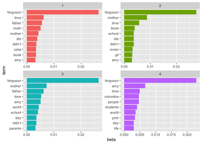
The figure shows that Ferguson is the defining character across all topics and the most prominent term. Further coherences can be drawn, such as the parents (“mother” and “father”) are among the most important terms across most topics. At the same time, however, we can also work out differences. For example, it can be seen that “columbia” (may be the university) plays a greater role in topic four. Furthermore, we can identify characters that occur exclusively in individual topics or are overrepresented, such as Vivian, Gil, Celia, and Noah.

We can systematically work out these topical differences, by taking the ratio of the corresponding betas. The following code programms in dplyr, which can be learned more about here.

log2ratio = function(first_topic, second_topic, topics_chapter){
  
  # Create the Beta Spread Table
  beta_spread = topics_chapter %>%
    mutate(topic = paste0("topic", topic)) %>%
    spread(topic, beta) %>%
    filter(!!sym(first_topic) > .001 | !!sym(second_topic) > .001) %>%
    mutate(log_ratio = log2(!!sym(first_topic) / !!sym(second_topic)))
  
  # Modify the Data
  top_n_beta_spreads = head(beta_spread[c('term','log_ratio')][order(-beta_spread[c('term', 'log_ratio')]$log_ratio),],n=5)

  tail_n_beta_spreads = tail(beta_spread[c('term', 'log_ratio')][order(-beta_spread[c('term', 'log_ratio')]$log_ratio),],n=5)
  
  top_beta_spread = top_n_beta_spreads %>% 
    add_row(term = tail_n_beta_spreads$term, log_ratio = tail_n_beta_spreads$log_ratio)
  top_beta_spread = top_beta_spread[order(top_beta_spread$log_ratio),]
  
  # Create the Plot
  par(mar=c(4,8,3,2)+.1)
  barplot(pull(top_beta_spread), horiz = TRUE, names.arg = top_beta_spread$term,las = 1, axes = FALSE,
        main = paste(as.character(first_topic), "/", as.character(second_topic)))
  axis(1,at=seq(round(min(top_beta_spread$log_ratio)),round(max(top_beta_spread$log_ratio)),50))
}

par(mfrow=c(3,2), cex=1.5)
log2ratio("topic1", "topic2", chapter_topics)
log2ratio("topic1", "topic3", chapter_topics)
log2ratio("topic1", "topic4", chapter_topics)
log2ratio("topic2", "topic3", chapter_topics)
log2ratio("topic2", "topic4", chapter_topics)
log2ratio("topic3", "topic4", chapter_topics)

We can see clear differences between the topics. For instance, topic2 appears to have a character aubrey that only plays a role in that particular storyline. Additionally, there are many more characters and distinctions we can make out due to the beta_spread. These differences help us as a reader, but also the model, to distinguish between different storylines.

So far we have considered each topic individually, trying to see the bigger picture by comparing all topics simultaneously. However, we may also take a look at one topic and its difference to all others. We do so by calculating the logarithmic ratio of one topic and the mean of the three others.

beta_spreads = function(first_topic, second_topic, 
                        third_topic, fourth_topic, topics_chapter){
  topics_chapter %>%
  mutate(topic = paste0("topic", topic)) %>%
  spread(topic, beta) %>%
  filter(!!sym(first_topic) > .001 | !!sym(second_topic) > .001 | !!sym(third_topic) > .001 | !!sym(fourth_topic) > .001)
}

beta_spread = beta_spreads("topic1", "topic2", "topic3", "topic4", chapter_topics)
beta_spread$log_avg1 = log2(beta_spread$topic1 / rowMeans(beta_spread[,3:5]))
beta_spread$log_avg2 = log2(beta_spread$topic2 / rowMeans(beta_spread[,c(2,4,5)]))
beta_spread$log_avg3 = log2(beta_spread$topic3 / rowMeans(beta_spread[,c(2,3,5)]))
beta_spread$log_avg4 = log2(beta_spread$topic4 / rowMeans(beta_spread[,2:4]))

plot_avg_spreads = function(df_spreads, topic){
  head_spreads = head(df_spreads[, c(1, 5+topic)][order(-df_spreads[, c(1, 5+topic)][,2]),],n=5)
  tail_spreads = tail(df_spreads[, c(1, 5+topic)][order(-df_spreads[, c(1, 5+topic)][,2]),],n=5)
  top_beta_spread = rbind(head_spreads, tail_spreads)
  top_beta_spread = top_beta_spread %>% map_df(rev)
  
  #par(mar=c(4,8,3,2)+.1)
  barplot(pull(top_beta_spread), horiz = TRUE, names.arg = top_beta_spread$term,las = 1, axes = FALSE,
          main = paste("Topic", topic, "/ Mean of Topic", toString(setdiff(c(1,2,3,4),topic))))
  axis(1,at=seq(round(min(top_beta_spread[,2])),round(max(top_beta_spread[,2])),50))
}

par(mfrow = c(2, 2), oma = c(1, 1, 1, 1), mar = c(5, 5, 5, 1), cex=1.5) 
plot_avg_spreads(beta_spread, topic = 1)
plot_avg_spreads(beta_spread, topic = 2)
plot_avg_spreads(beta_spread, topic = 3)
plot_avg_spreads(beta_spread, topic = 4)

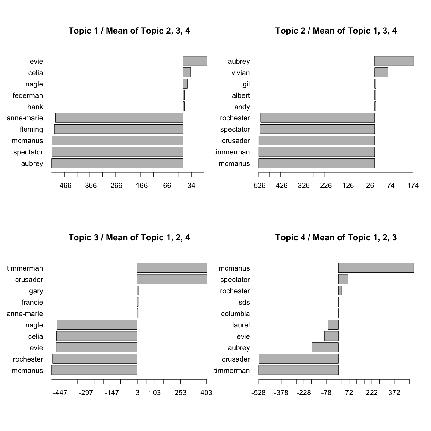
Using this graphic we can clearly see which terms make up a topic. For example, we see that Evie and Celia are characters from topic 1, while Aubrey and Vivian seem to be characters from topic 2. By comparing one topic with all the others simultaneously (and direclty), we can draw conclusions about the uniqueness of individual terms (words) in topics.

After examining the varying terms and their betas in depth, we may take a closer look at the per-document classification. How well does the LDA model assign the chapters to their respective storyline?

Per-document classification

To each chapter there are four per-document-per-topic probabilities (topic 1, 2, 3 and 4).

chapters_gamma = tidy(chapters_lda, matrix = "gamma")

Thus, we can see the probabilities with which the model assigns each chapter to a topic.

chapters_gamma[chapters_gamma$document == "Storyline-1_Chapter-1",]

## # A tibble: 4 x 3
##   document              topic      gamma
##   <chr>                 <int>      <dbl>
## 1 Storyline-1_Chapter-1     1 0.00000651
## 2 Storyline-1_Chapter-1     2 0.854     
## 3 Storyline-1_Chapter-1     3 0.146     
## 4 Storyline-1_Chapter-1     4 0.00000651

The model believes the first chapter of the first storyline belongs to the second topic. We may seperate the chapters from the storylines.

chapters_gamma = chapters_gamma %>%
  separate(document, c("title", "chapter"), sep = "_", convert = TRUE)

And then illustrate the per-document-per-topic probability for all chapters.

chapters_gamma %>%
  mutate(title = reorder(title, gamma * topic)) %>%
  ggplot(aes(factor(topic), gamma)) +
  geom_boxplot() +
  facet_wrap(~ title)

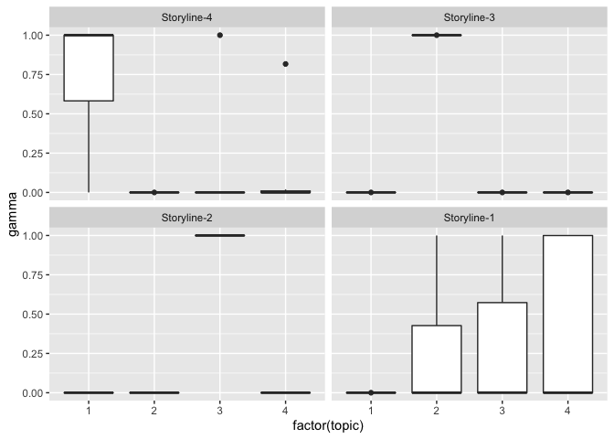
From the plot we can see that Storyline-2, Storyline-3 and Storyline-4 are classified well, Storyline-1, however, is ambiguous. To get a better understanding why the first storyline is harder to be classified, we may take a closer look at the classified chapters. chapter_classifications gives away the probabilities with which the model assigns each chapter to a topic.

chapter_classifications = chapters_gamma %>%
  group_by(title, chapter) %>%
  top_n(1, gamma) %>%
  ungroup() %>%
  arrange(gamma)

book_topics = chapter_classifications %>%
  count(title, topic) %>%
  group_by(title) %>%
  top_n(1, n) %>%
  ungroup() %>%
  transmute(consensus = title, topic)

After examining the chapters and their classification, we may also take a look at the terms (words) and their classification. This may be done using augment from the package broom.

assignments = augment(chapters_lda, data = chapters_dtm)

assignments = assignments %>%
  separate(document, c("title", "chapter"), sep = "_", convert = TRUE) %>%
  inner_join(book_topics, by = c(".topic" = "topic"))

Adding the consensus (books assigned to) to the assignments tibble lets us examine the relationship between words and their misclassification to other chapters. It may be visualized for clarification using ggplot.

assignments %>%
  count(title, consensus, wt = count) %>%
  group_by(title) %>%
  mutate(percent = n / sum(n)) %>%
  ggplot(aes(consensus, title, fill = percent)) +
  geom_tile() +
  scale_fill_gradient2(high = "red", label = percent_format()) +
  theme_minimal() +
  theme(axis.text.x = element_text(angle = 90, hjust = 1),
        panel.grid = element_blank()) +
  labs(x = "Book words were assigned to",
       y = "Book words came from",
       fill = "% of assignments")

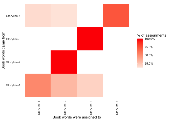
We can see that all words that came from Storyline-3 and Storyline-2 were correctly classified to their storyline. Words from Storyline-1 and Storyline-4 were mainly correctly classified, but carried some minsinterpretation as well.

So far we have given the model the whole chapter for classification. But we may ask, how many words (or pages) does the model need to accurately classify the chapter?

The following code takes n words (stepSize), creates an LDA model and subsequently classifies the sub-chapter. This is done for all chapters across the book.

Paragraph2Topic = function(lda_obj=chapters_lda , df, doc="Storyline-1_Chapter-1", start=100, end = 1600){
  df2 = subset(df, document == doc)#paste0("Storyline-",storyline,"_Chapter-",chapter)
  df2 = df2[start:end,]
  
  word_counts2 = df2 %>% anti_join(stop_words) %>% count(document, word, sort = TRUE) 
  
  
  chapters_dtm2 = word_counts2 %>%
    cast_dtm(document, word, n) 
  
  lda_inf <- posterior(lda_obj, chapters_dtm2) 
  return(lda_inf)
}

all_chapters = function(seed = 123, stepSize = 1000){
  
  set.seed(seed) # Set Seed
  
  docs = unique(df$document) # List of 22 Chapters
  chapter_lengths = table(df$document) # Lengths of Chapters
  chapter_lengths = round(chapter_lengths, -3)-1000 # Rounds the chapters_lengths down, so the last iteration does not overshoot the length
  nmbrRows = sum(chapter_lengths/stepSize) # To pre-allocate the space, the number of rows must be known
  df_chapters = data.frame(matrix(ncol = 5, nrow = nmbrRows)) # Initialize and pre-allocate the data.frame
  df_chapters = df_chapters %>% rename(Chapter = X1, StepSize = X2, Window = X3, Classified = X4, Correct = X5) # Rename the data.frame
  iteration = 1 # Counter
  
  for (j in 1:length(chapter_lengths)) { # Outer loop: Loops over the Chapters 
    d = docs[j] # Define the doc
    sequ = seq(1,chapter_lengths[j], stepSize) # Creates a sequence, given the length of the respective chapter
    for (i in 1:length(sequ)) { # Inner loop: Loop through the single chapers
      s = sequ[i] # Takes the given starting point
      lda_inf=suppressMessages(Paragraph2Topic(chapters_lda ,df,doc=d,start=s, end = s+stepSize)) # Suppresses the "Join by = " message
  
      df_chapters$Chapter[iteration] = d # Assign the chapter name
      df_chapters$StepSize[iteration] = stepSize # Assign the step size
      df_chapters$Window[iteration] = i # Assign the window number
      df_chapters$Classified[iteration] = which.max(lda_inf$topics) # Classifications 
      df_chapters$Correct[iteration] = book_topics$topic[as.integer(substr(docs[j], 11,11))] # Corrects
      
      iteration = iteration + 1 # Increase the counter
    }
  }
  return(df_chapters)
}

We may call the function using a stepSize of 100. That is, we only provide the model with 100 words and challenge it to correctly classify it. The second line gives us the Accuracy, the correctly classified chapters, divided by all.

df_chapters = all_chapters(stepSize = 100)
sum(df_chapters$Classified == df_chapters$Correct) / length(df_chapters$Classified)

## [1] 0.746988

In order to create the confusion matrix, we need to adjust the data.frame.

# Adapt the data.frame to make it compatible with the Confusion Matrix code
df_chapters_CM = df_chapters %>%
  separate(Chapter, c("Title", "Chapter"), sep = "_", convert = TRUE) %>%
  inner_join(book_topics, by = c("Classified" = "topic"))

Now we can take the slightly adjusted code from above, to create a confusion matrix.

# Confusion Matrix
df_chapters_CM %>%
  count(Title, consensus) %>%
  group_by(Title) %>%
  mutate(percent = n / sum(n)) %>%
  ggplot(aes(consensus, Title, fill = percent)) +
  geom_tile() +
  scale_fill_gradient2(high = "red", label = percent_format()) +
  theme_minimal() +
  theme(axis.text.x = element_text(angle = 90, hjust = 1),
        panel.grid = element_blank()) +
  labs(x = "Correct Chapters",
       y = "Assigned Chapters",
       fill = "% of assignments")

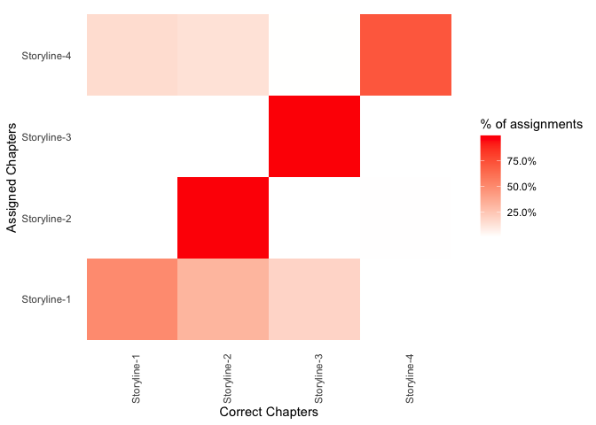
We can see that all chapters that came from Storyline-2 and Storyline-3 were correctly classified to their storyline. Chapters from Storyline-1 and Storyline-4 were mainly correctly classified, but carried some minsinterpretation as well. Thus, we may ask what these misinterpretations were.

Mistaken words

By comparing the title (true chapter) with the consensus (classified chapter) we can spot differences.

mistakes = assignments %>%
  filter(title != consensus)

mistakes = mistakes %>%
    count(title, consensus, term, wt = count) %>%
    ungroup() %>%
    arrange(desc(n))

mistakes

## # A tibble: 14,714 x 4
##    title       consensus   term         n
##    <chr>       <chr>       <chr>    <dbl>
##  1 Storyline-1 Storyline-2 ferguson   278
##  2 Storyline-4 Storyline-1 ferguson   221
##  3 Storyline-1 Storyline-3 ferguson   190
##  4 Storyline-4 Storyline-2 ferguson   164
##  5 Storyline-1 Storyline-2 amy         95
##  6 Storyline-1 Storyline-3 mother      80
##  7 Storyline-1 Storyline-2 mother      71
##  8 Storyline-4 Storyline-2 mother      66
##  9 Storyline-1 Storyline-2 father      64
## 10 Storyline-4 Storyline-1 father      62
## # … with 14,704 more rows

The main character ferguson was the character most often misclassified, which does not come as a surprise, as he spans across all storylines. Other often wrongly classified characters are the mother and father, as well as amy.

Note: You may find this Blog Post on R-Bloggers.com as well.

References

David M. Blei. Probabilistic topic models. Communications of the ACM, Vol. 55 No. 4, Pages 77-84, 2012.

Julia Silge and David Robinson. Text Mining with R, O’Reilly, 2020.

LDA: 4321

Table of Contents