Stacked Regressions
Reproducible Research
In a recent paper on Stacked regressions and structured variance partitioning for interpretable brain maps, the authors argue that stacking frequently (and substantially) outperforms more traditional approaches such as concatenated regression models, particularly when it comes to feature attribution and variance explanation in high-dimensional settings.
A central piece of evidence for this claim is Figure 4 of the paper. The figure is striking: across a wide range of simulated scenarios, stacking appears to outperform concatenation most of the time, often by a large margin. Visually, it suggests that stacking not only improves predictive performance but also delivers markedly superior estimates of the unique contribution of feature blocks—a claim with important methodological implications for applied work.
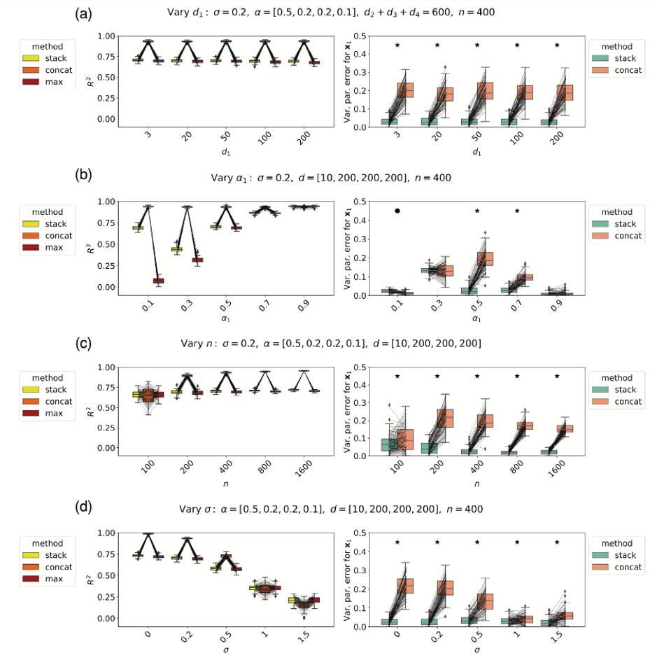
Because of its prominence and apparent robustness, Figure 4 strongly shapes the reader’s takeaway from the paper. It effectively serves as a flagship result supporting the narrative that stacking is the preferred method for feature attribution in complex, high-dimensional problems.
However, as I discovered while carefully examining the accompanying code, the quantity plotted in Figure 4 is not the partial (or unique) R² it is interpreted as, but rather a marginal R². This distinction is not cosmetic: it changes the scientific question the figure answers. Over the subsequent months, I communicated this issue to the authors, who acknowledged the formula error, but are less convinced that Figure 4 needs to be replaced.
In what follows, I explain why this position is untenable. I will argue that Figure 4, as currently presented, does not support the claims it is used to justify—regardless of whether the simulated feature blocks are correlated or not. The problem is not subtle, and it goes to the heart of what the figure is supposed to demonstrate.
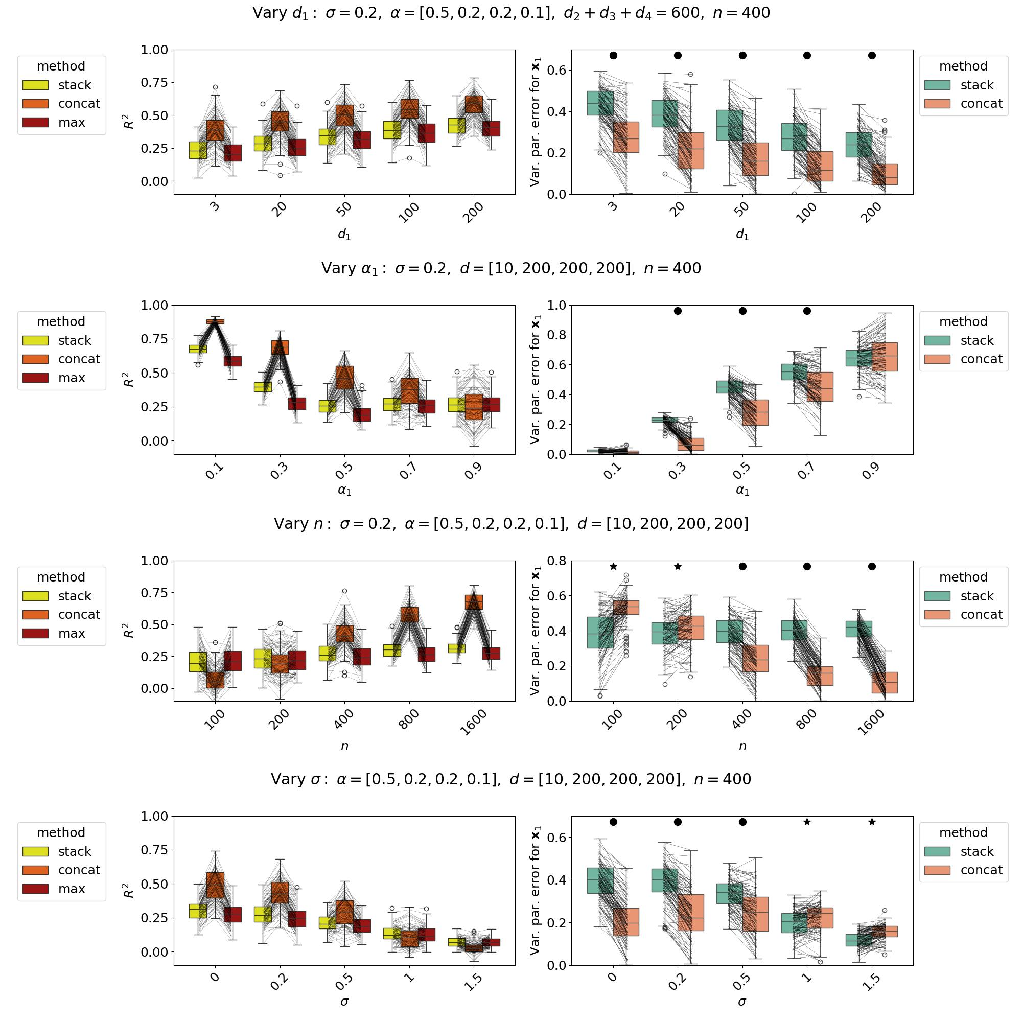
For completeness, I have recreated Fig. 4 using the by now hopefully correct partial R², and its message is dramatically different:
1. What Figure 4 is claimed to show vs. what it actually shows
What the paper claims Fig. 4 demonstrates
Across the paper, Fig. 4 plays a very specific rhetorical role:
- It is not “just a toy simulation”.
- It is presented as evidence that stacking outperforms concatenation, especially for feature attribution / variance partitioning.
- The y-axis is repeatedly interpreted as “unique contribution” / “partial R²” of a feature space.
So Fig. 4 is not neutral: it visually communicates robust superiority.
2. The key technical fact: the quantity plotted was not partial R²
- the intended estimand was unique / partial variance, and
- the existing implementation did not correctly isolate it.
3. Why “correlation = 0” does not rescue Figure 4
The key point:
Marginal R² ≠ Partial R² even when feature spaces are independent in the DGP.
Why?
-
Stacking and concatenation induce dependence at the prediction stage
- Even if \(X_1 \perp X_2\) in the data-generating process,
- stacked predictions \(\hat y_1, \hat y_2\) are not orthogonal in finite samples,
- especially under regularization, cross-validation, and high (p/n).
-
Marginal R² systematically over-credits flexible models
- Marginal R² measures “how much variance can be explained when used alone”.
- Stacking is designed to maximize predictive alignment with (y).
- So marginal R² will mechanically favor stacking, even in regimes where it adds no unique information.
-
Therefore Fig. 4 answers the wrong question
- It answers: “Which method fits y better marginally?”
- But it is interpreted as: “Which method recovers unique contributions better?”
This mismatch exists even at correlation = 0.
4. Fig. 4 was already inconsistent with the text
- Fig. 4 does not match the textual description.
- The only proposed “fix” is reinterpretation, not recomputation.
The numerical dominance itself is an artifact of using marginal instead of partial R².
So the problem is not just labeling.
5. Core argument
Figure 4 must be rerun because it plots the wrong estimand. Even in the zero-correlation setting, marginal R² does not measure unique contribution and therefore systematically exaggerates the advantage of stacking.
Supporting points
- The paper claims to study structured variance partitioning.
- Partial R² is the only estimand aligned with that goal.
- The code originally computed marginal R² (acknowledged in June).
- Using marginal R² favors stacking by construction.
- Therefore Fig. 4 is methodologically invalid, not just “parameter-dependent”.
Even under the assumption, that for zero correlation in the simulated data, \(\text{marginal } R^2 = \text{partial } R^2.\) Figure 4 is still problematic for the paper as written.
1. Figure 4 is interpreted as evidence of general superiority
Figure 4 is not presented as:
“a very special, degenerate case with no correlation where methods coincide.”
Instead, it is used to support claims like:
- stacking outperforms concatenation most of the time,
- stacking provides better feature attribution,
- results are robust across high-dimensional regimes.
So even if Fig. 4 were correct for the zero-correlation DGP, its rhetorical role far exceeds that scope.
2. Zero correlation is a knife-edge case
Under your hypothetical:
-
Zero correlation is exactly the case where
- marginal = partial,
- variance attribution is trivial,
- identifiability issues disappear.
That makes Fig. 4 a knife-edge scenario, not a representative one.
Consequence
Using it as flagship evidence is misleading, because:
- any deviation from zero correlation invalidates the interpretation,
- the reader is not alerted that the result depends on a very special case.
So the figure may be numerically correct, but scientifically fragile.
3. The figure no longer supports the stated contribution
The paper’s contribution is about:
- structured variance,
- overlapping or correlated feature spaces,
- realistic high-dimensional settings.
But under your hypothetical assumption, Fig. 4 is actually showing:
“When there is no correlation, stacking predicts better.”
That is:
- unsurprising,
- not about variance partitioning,
- not evidence of better feature attribution.
So Fig. 4 does not support the claimed methodological advance, even if the numbers are “right”.
4. Internal inconsistency remains
Even in the hypothetical world where marginal = partial at correlation = 0:
- The text discusses correlation and structured variance.
- Figure 4 implicitly relies on correlation = 0 to be interpretable.
- The dependence of the result on this assumption is neither highlighted nor tested.
This is still an internal inconsistency between figure, estimand, and narrative.
5. Summary
Even if marginal and partial R² coincide at zero correlation, Figure 4 remains problematic because it is a knife-edge special case that is used to support broad claims about feature attribution in structured, high-dimensional settings. The figure is therefore either misleading in scope or irrelevant to the main contribution.
6. Logical structure
| Assumption | Conclusion |
|---|---|
| marginal ≠ partial | Fig. 4 is wrong |
| marginal = partial at ρ = 0 | Fig. 4 is misleading |
| ρ ≠ 0 (realistic case) | Fig. 4 is invalid |
So in every logically possible case, Fig. 4 cannot stand as-is.